Regression
Overview
Teaching: 60 min
Exercises: 30 minQuestions
PDF version + exercises
1. Regression Introduction
Regression analysis is a conceptually simple method for investigating functional relationships among variables.
Regression Analysis By Example by Samprit Chatterjee, Ali S. Hadi and Bertram Price available online from the MQ library.
EXAMPLE: A new Real Estate agent in Macquarie, ACT wants to come up with a sale price for a house based on some physical characteristics.
She has some past sales data on houses that sold in 2018. Note that I have de-identified the records by removing the addresses.
library(tidyverse)
library(ggpubr)
library(olsrr)

theme_set(theme_bw())

houses <- read_csv(file.path("..", "data", "Macquarie2018.csv"))
houses
# A tibble: 15 x 8
   Contract_Date  Price Block_Size Bedrooms Bathrooms Ensuites Garages
   <chr>          <dbl>      <dbl>    <dbl>     <dbl> <lgl>      <dbl>
 1 12/10/2018    605000        780       NA        NA NA            NA
 2 14/07/2018    645000        761        4         1 NA             2
 3 22/05/2018    670000        433        3         1 NA             0
 4 15/01/2018    682000       1173       NA        NA NA            NA
 5 27/11/2018    700000        698       NA        NA NA            NA
 6 24/09/2018    710000        971       NA        NA NA            NA
 7 24/01/2018    721000        453        3         2 NA             0
 8 2/06/2018     723000        850        3         1 NA             2
 9 5/12/2018     785000        871        3         1 NA             1
10 2/11/2018     800000        929        3         1 NA            NA
11 28/02/2018    848000       1039       NA        NA NA            NA
12 15/02/2018    860000        941        3         1 NA             1
13 21/09/2018    868000        808        3         1 NA             1
14 8/12/2018     877500       1179        4         2 NA             2
15 9/11/2018     900000        808       NA        NA NA            NA
# ... with 1 more variable: Carports <dbl>
Response (Dependent variable, Outcome variable): Price ($Y$)
Predictors (Explanatory variables, independent variables, covariates, regressors): Block Size ($X_1$), Bedrooms ($X_2$), Bathrooms ($X_3$), Ensuites ($X_4$), Garages ($X_5$), Carports ($X_6$).
Regression Model:
This is used as an approximation to the true relationship between $Y$ and $X_1$, $X_2$, $X_3$, $X_4$, $X_5$, $X_6$.
The function $f(X_1,X_2,X_3,X_4,X_5,X_6)$ describes relationship between $Y$ and $X_1$, $X_2$, $X_3$, $X_4$, $X_5$, $X_6$.
$\varepsilon$ is assumed to be random error representing the discrepancy between $Y$ and $f(X_1,X_2,X_3,X_4,X_5,X_6)$.
Linear regression model:
The $\beta_0$, $\beta_1$, $\beta_2$,$\cdots$, $\beta_6$ are called regression parameters or coefficients, are unknown constants that need to be estimated from the data.
1.2 STEPS IN REGRESSION ANALYSIS
Statement of the problem
Question/s to be addressed by the analysis must be carefully thought out.
EXAMPLE: Determine the sale price for some houses in Macquarie.
Selection of potentially relevant variables
Select a set of variables that are thought to explain or predict the response variable. Usually use those suggested by experts in the area of study.
EXAMPLE: The Real Estate Agent might think Block Size strongly influences house sale price.
Usually record data as follows
Each row corresponds to an observation. Each column corresponds to a variable. For each observation we have one value for the response variable and one value for each of the $p$ predictors.
We can classify the variables as quantitative or qualitative (categorical) and further divide categorical variables as being ordinal or nominal (no ordering in the categories).
EXAMPLE: In the Macquarie Real Estate example, except for Contract Date, all variables can be considered to be quantitative.
Model specification
Need to select the form of the function $f(X_1,X_2,\cdots,X_p)$. Could be specified initially by experts in the field of study based on their knowledge or judgements (objective and / or subjective). Hypothesized model can be rejected or not rejected by the analysis of the collected data.
Only the form of the function $f(X_1,X_2,\cdots,X_p)$ needs to be specified. The function may be classified as linear or nonlinear. Do the regression parameters enter the equation linearly or nonlinearly?
Various Classifications of Regression Analysis
| Type of Regression | Conditions |
|---|---|
| Univariate | Only one quantitative response variable |
| Multivariate | Two or more quantitative response variables |
| Simple | Only one predictor variable |
| Multiple | Two or more predictor variables |
| Linear | All parameters enter the equation linearly, possibly after transformation of the data |
| Nonlinear | The relationship between the response and some of the predictors is nonlinear or some of the parameters appear nonlinearly, but no transformation is possible to make the parameters appear linearly |
| Analysis of Variance | All predictors are qualitative variables |
| Analysis of Covariance | Some predictors are quantitative variables and others are qualitative variables |
| Logistic | The response variable is qualitative |
(Page 15, Regression Analysis by Example, Third Edition by Samprit Chatterjee, Ali S. Hadi and Bertram Price (2000).)
Choice of fitting model
The Least Squares method is most commonly used. Under certain conditions this method produces estimators with desirable properties. We will use least squares or weighted least squares most of the time.
Model fitting
Estimation of regression parameters or fitting the model to the collected data using the chosen method of fitting. It is usual to denote estimates of the regression parameters $\beta_0,~\beta_1,~\beta_2,\cdots,~\beta_p$ by $\hat{\beta}_0,~\hat{\beta}_1,~\hat{\beta}_2,\cdots,~\hat{\beta}_p$.
If fitting a multiple linear regression to the data the estimated regression becomes Note that $\hat{Y}$ (said Y-hat) is called the fitted value.
The i-th fitted value is
We can use ($\text{*}$) to predict the response variable for any values of the predictor variables not observed in our data, the obtained $\hat{Y}$ is called the predicted value.
Do not predict the response variable for a set of predictor variables outside the range of the data.
Model validation and criticism
The assumptions made about the data to fit a particular model need to be checked. This can only be done after the model has been fitted to the data.
If model assumptions do not hold the analysis produced (we will use the lm function in R)
will not be valid. There is no point looking at p-values if the model assumptions do not hold.
You always need to check that the model assumptions hold when fitting a model to the data.
Using the chosen model(s) for the solution to the posed problem
EXAMPLE: Suppose that the new Macquarie Real Estate Agent has the feeling that house price is closely related to block size.
I have the data saved in the file Macquarie2018.csv that you can download from the following
location ….
I use the readr package which is part of the Tidyverse to get the data into R. Make sure you
change your Directory in R to the one where you have saved this data set. Google readr r for
documentation for more details about this package.
ggplot(houses, aes(x = Block_Size, y = Price)) +
    geom_point()
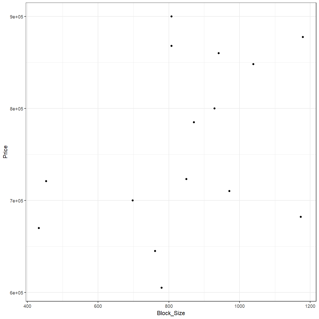
The agent feels that the relationship looks linear. A simple linear regression is fitted to the data by a first year Statistics student. The simple linear regression model is
with $E(\varepsilon_i)=0$, $Var(\varepsilon_i)=\sigma^2$ and
$Cov(\varepsilon_i,\varepsilon_j)=0$. We can also assume that $\varepsilon_i \sim N(0,\sigma^2)$
(i.e., the $\varepsilon$ is normally distributed with zero mean and constant variance
$\sigma^2$).
This normality assumption is not needed for the least squares estimation but it is necessary
for the standard confidence intervals and hypothesis tests.
We fit the model by estimating values for the parameters $\beta_0$, $\beta_1$ and $\sigma^2$.
houses_fit <- lm(Price ~ Block_Size, data = houses)
To get the estimated values of $\beta_0$ and $\beta_1$:
houses_fit
Call:
lm(formula = Price ~ Block_Size, data = houses)

Coefficients:
(Intercept)   Block_Size
     616624          169
To get more detailed output from the model fitted to the data:
summary(houses_fit)
Call:
lm(formula = Price ~ Block_Size, data = houses)

Residuals:
    Min      1Q  Median      3Q     Max
-143435  -53988   21187   58718  146833

Coefficients:
            Estimate Std. Error t value Pr(>|t|)
(Intercept) 616624.3    98136.8   6.283 2.82e-05 ***
Block_Size     169.0      112.6   1.501    0.157
---
Signif. codes:  0 '***' 0.001 '**' 0.01 '*' 0.05 '.' 0.1 ' ' 1

Residual standard error: 90700 on 13 degrees of freedom
Multiple R-squared:  0.1476,	Adjusted R-squared:  0.08207
F-statistic: 2.252 on 1 and 13 DF,  p-value: 0.1574
More importantly, before looking at any p-values, look at the diagnostic plots.
par(mfrow = c(2, 2))
plot(houses_fit)
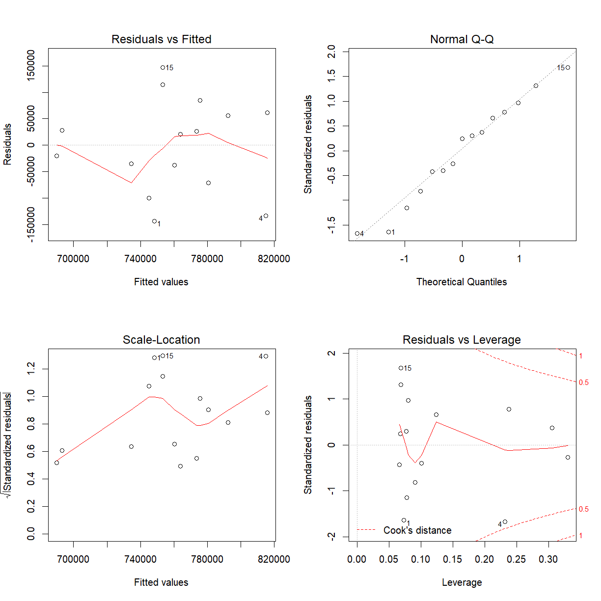
For you to be satisfied that the model is adequate and that you can proceed to make inference the Residual vs Fitted values plot should look like a random scatter about zero and the Normal Q-Q plot should look linear. Even if we fit a multiple linear regression we still look at these two plots to assess model adequacy.
Suppose you thought the model is adequate (it isn’t so).
The regression equation is
where $Y=$ Price and $x=$ Block Size.
You see that the Adjusted R-Squared is 0.08207 and that the F Statistic p-value is 0.1574, if the model is adequate and the normality assumption holds you can make the following statements:
The Block Size accounts for 8.2% of the variation in Price. The regression is not significant (p-value=0.157).
1.3 COVARIANCE AND CORRELATION COEFFICIENT
We are interested in studying the relationship between a response variable $Y$ and a single predictor $X$.The covariance between $Y$ and $X$ measures the direction of the linear relationship between $Y$ and $X$ but tells us nothing about the strength of the relationship since it changes if we change the unit of measurement. If $Cov(Y,X)>0$ then there is a positive relationship between $Y$ and $X$ but if $Cov(Y,X)<0$ the relationship is negative.
The correlation coefficient between $Y$ and $X$ is scale invariant so it measures both the direction and strength of the linear relationship between $Y$ and $X$.
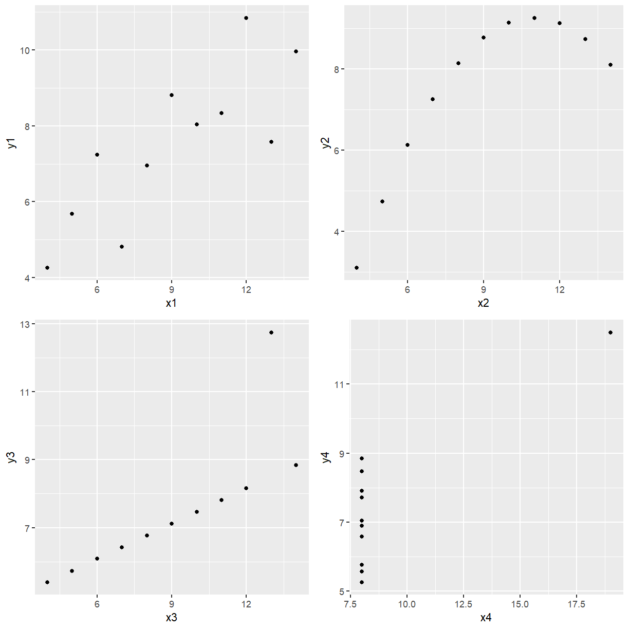
EXAMPLE: Anscomb (1973) used four data sets to illustrate the importance of investigating the data using scatter plots and not relying totally on the correlation coefficient. The four data sets are given below. Explore the data graphically and obtain the correlation coefficient for each data set. ($r^2=\frac{\sum(x_i-\bar{x})(y_i-\bar{y})}{\sum(x_i-\bar{x})^2\sum(y_i-\bar{y})^2)}$)
The file Anscombe.csv contains this data.
library(tidyverse)
library(readr)

anscomb <- read_csv(file.path("..", "data", "Anscomb.csv"))
anscomb
# A tibble: 11 x 8
      x1    y1    x2    y2    x3    y3    x4    y4
   <dbl> <dbl> <dbl> <dbl> <dbl> <dbl> <dbl> <dbl>
 1    10  8.04    10  9.14    10  7.46     8  6.58
 2     8  6.95     8  8.14     8  6.77     8  5.76
 3    13  7.58    13  8.74    13 12.7      8  7.71
 4     9  8.81     9  8.77     9  7.11     8  8.84
 5    11  8.33    11  9.26    11  7.81     8  8.47
 6    14  9.96    14  8.1     14  8.84     8  7.04
 7     6  7.24     6  6.13     6  6.08     8  5.25
 8     4  4.26     4  3.1      4  5.39    19 12.5
 9    12 10.8     12  9.13    12  8.15     8  5.56
10     7  4.82     7  7.26     7  6.42     8  7.91
11     5  5.68     5  4.74     5  5.73     8  6.89
Now we want to see what each data set looks like.
p1 <- ggplot(anscomb, aes(x = x1, y = y1)) + geom_point()
p2 <- ggplot(anscomb, aes(x = x2, y = y2)) + geom_point()
p3 <- ggplot(anscomb, aes(x = x3, y = y3)) + geom_point()
p4 <- ggplot(anscomb, aes(x = x4, y = y4)) + geom_point()

ggarrange(p1, p2, p3, p4, ncol = 2, nrow = 2)
Base R has the cor function to produce correlations and the cov function to produce
covariances. The default is Pearson’s correlation.
cor(anscomb$x1, anscomb$y1)
[1] 0.8164205
cor(anscomb$x2, anscomb$y2)
[1] 0.8162365
cor(anscomb$x3, anscomb$y3)
[1] 0.8162867
cor(anscomb$x4, anscomb$y4)
[1] 0.8165214
To two decimal places, all 4 sets of data have
0.82
correlation yet the plots don’t all look linear. Just because you have a high correlation is not
a sufficient reason to fit a straight line to the data. Even though Data Set 2 has high positive
correlation it is obvious from the plot of y2 vs x2 that a perfect nonlinear relationship
describes the relationship between the two variables better. Looking at the plot of y3 versus
x3 it is obvious if it wasn’t for the second last data point the relationship would be
perfectly linear with a positive slope. Look at the last plot, if it wasn’t for the point on its
own there would be no relationship between y4 and x4, such a point is called highly
influential because if it was removed the curve fitted would be very different. Only the plot of
y1 versus x1 could be considered to be approximately linear.
1.4 THE SIMPLE LINEAR REGRESSION MODEL
If the scatter plot of response variable ($Y$) against predictor variable ($X$) is approximately linear we use it to study the relationship between $Y$ and $X$.The response variable $Y$ is of primary importance.
Model: $y_i=\beta_0+\beta_1x_i+\varepsilon_i$ with $E(\varepsilon_i)=0$, $Var(\varepsilon_i)=\sigma^2$ and $Cov(\varepsilon_i,\varepsilon_j)=0$.
This model represents a linear relationship between the variables $x$ and $y$, with uncorrelated errors with constant variance. The errors are not mistakes but represent the variation in the response that is not accounted for by the explanatory variable. We can also assume that $\varepsilon_i \sim N(0,\sigma^2)$ but this assumption is not needed for the least squares estimation but it is necessary for the standard confidence intervals and hypothesis tests. We fit the model by estimating values for the parameters $\beta_0$ (intercept), $\beta_1$ (slope) and $\sigma^2$.
Now
which means “The expected value of the random variable $Y$, given that $X$ is fixed at the value $x$, is equal to $\beta_0+\beta_1 x$”.
1.4.1 Least squares estimation
The least squares estimates of $\beta_0$ and $\beta_1$ are those values $\hat{\beta}_0$ and $\hat{\beta}_1$ that minimise the ‘residual sum of squares’ function
The least squares estimates $\hat{\beta}_0$ and $\hat{\beta}_1$ are $\hat{\beta}_0=y-\beta_1 \bar{x}$, $\beta_1=S_{XY}/S_{XX}$ where $S_{XX}=\sum (x_i-\bar{x})^2$, $S_{XY}=\sum (x_i-\bar{x})(y_i-\bar{y})$, and $S_{YY}=\sum (y_i-\bar{y})^2$.
We define the fitted values by $\hat{y}_i=\hat{\beta}_0+\hat{\beta}_1 x_i$, and residuals by $e_i=\hat{y}_i-y_i$.
We estimate the variance $\sigma^2$ by
where $SSE=\sum e_i^2=\sum(y_i-\hat{y}_i)^2=(S_{YY}-\hat{\beta}_1S_{XY})$.
1.4.2 Properties of the estimators
$E(\hat{\beta}_1)=\beta_1$,
$Var(\hat{\beta}_1)=\frac{\sigma^2}{S_{XX}} (1)$,
$E(\hat{\beta}_0)=\beta_0$,
$Var(\hat{\beta}_0)=\sigma^2(\frac{1}{n}+\frac{\bar{x}^2}{S_{XX}}) (2)$,
$E(\hat{y}_i)=\beta_0+\beta_1 x_i$,
$Var(\hat{y}_i)=\sigma^2(\frac{1}{n}+\frac{(x_i-\bar{x})^2}{S_{XX}}).$
The variance consists of two parts:
The first reflects the fact that the fit is based on a line obtained from a sample of $n$ values.
The second depends on how far the x-value is from the average of the $x$’s, and reflects the fact that the regression line is most accurate near the average of the $x$’s, and least accurate at the extremes.
Replacing $\sigma^2$ in (2) and (1) by $\hat{\sigma}^2$ we get unbiased estimators of the variances of $\hat{\beta}_0$ and $\hat{\beta}_1$.
1.4.3 Tests of hypotheses
Hypothesis tests concerning the slope
Test $H_0:\beta_1=\beta_1^0$ against $H_1:\beta_1 \neq \beta_1^0$ using test statistic $t_1=\frac{\hat{\beta}_1-\beta_1^0}{s.e.(\hat{\beta}_1)}$ which has a $t_{n-2}$ distribution if H_0 is true.
Rejection region: $|t| \geq t_{n-2;\alpha/2}$ where $\alpha=0.05$ if testing at 5% significance level.
P-value: p-value>$\alpha$
EXAMPLE: Regressing Price on Block Size. Done earlier, saved as houses_fit.
summary(houses_fit)
Call:
lm(formula = Price ~ Block_Size, data = houses)

Residuals:
    Min      1Q  Median      3Q     Max
-143435  -53988   21187   58718  146833

Coefficients:
            Estimate Std. Error t value Pr(>|t|)
(Intercept) 616624.3    98136.8   6.283 2.82e-05 ***
Block_Size     169.0      112.6   1.501    0.157
---
Signif. codes:  0 '***' 0.001 '**' 0.01 '*' 0.05 '.' 0.1 ' ' 1

Residual standard error: 90700 on 13 degrees of freedom
Multiple R-squared:  0.1476,	Adjusted R-squared:  0.08207
F-statistic: 2.252 on 1 and 13 DF,  p-value: 0.1574
If the model assumptions and normality assumption hold (which they don’t) we would conclude that since the p-value associated with the coefficient of Block Size is 0.157 so we do not reject the hypothesis $H_0:\beta_1=0$ in favour of $H_1:\beta_1 \neq 0$. In a report you would write something like “Insufficient evidence to support house prices being influenced by block sizes in Macquarie (p=0.157)”. Different journals have different requirements for reporting statistical results. You need to make sure you extract all the information for the style you have to use, for example APS style requires more (see https://apastyle.apa.org/ or do a Google search if the information isn’t there).
A Test Using Correlation Coefficient
Test $H_0:\rho=0$ versus $H_1:\rho \neq 0$ using test statistic $t=\frac{r}{\sqrt{(1-r^2)/(n-2)}}$ which has a $t_{n-2}$ distribution when $H_0$ is true.
This is also equivalent to testing $H_0:\beta_1 = 0$ against $H_1:\beta_1 \neq 0$ in a simple linear regression of $Y$ on $X$.
Hypothesis tests concerning the intercept
Test of $H_0:\beta_0=\beta_0^0$ against $H_1:\beta_0\neq \beta_0^0$ is based on $t_0=\frac{\hat{\beta}_0-\beta_0^0}{s.e.(\hat{\beta}_0)}$ which has a $t_{n-2}$ distribution if $H_0$ is true.
EXAMPLE:
Back to regressing Price on Block Size. The previous output had a p-value of 2.82e-05 (0.0000282) so if the model is adequate and normality assumption holds you would conclude that the intercept is significant (testing $H_0:\beta_0=0$ against $H_1:\beta_0\neq 0$).
Confidence Intervals and Prediction Intervals
Sometimes you don’t just want to quote a p-value but provide a confidence interval. This output
is available from lm in R. For more details see
https://stat.ethz.ch/R-manual/R-devel/library/stats/html/confint.html
confint(houses_fit)
                   2.5 %      97.5 %
(Intercept) 404612.65155 828635.9089
Block_Size     -74.30034    412.2767
This is giving you a default 95% confidence interval for the intercept and slope. You would write something like the “95% confidence interval is (-74.3,412.3) for Block Size”, since the confidence interval contains zero there is insufficient evidence that Block Size influences Price. Again, only report this information if the model assumptions hold (residual versus fitted values plot looks like a random scatter about zero and the normal probability plot looks linear).
To get prediction intervals you need to create a new data frame that sets the Block Size. The example below is only getting a default 95% prediction interval for a block of size 800 m2.
newdata <- data.frame(Block_Size = 800)
predict(houses_fit, newdata, interval = "predict")
       fit      lwr      upr
1 751814.8 549136.4 954493.3
For details on how confidence interval or prediction intervals are calculated from formula look at CHP which is available online from the library.
If the model assumptions hold then the predicted price for a block size of 800 m2 is $751,814.8 and the 95% prediction interval is ($549,136.4, $954,493.3).
1.4.6 Analysis of variance (ANOVA)
ANOVA is a technique where the total variability in a set of data is split up into components assigned to various sources of variability:
The total variability is measured by $SS_{yy}=\sum (y_i-y)^2$, also called SST or ‘total sums of squares’.
The SST can be split into SSR or ‘regression sums of squares’ and SSE or ‘residual sums of squares’ as follows:
SST = SSR + SSE
If SSR is large compared to SSE, the regression explains most of the variability in $Y$ and hence is worthwhile.
If SSR is small compared to SSE, the regression is not explaining much of the variability in $Y$.
The comparisons must take into account the degrees of freedom for each component, and so are made using mean squares (sums of squares divided by degrees of freedom), denoted by MS. The test for significance of the regression is carried out by comparing the ratio of Regression Mean Square (MSR) and RMS to the $F_{1,n-2}$ distribution. To carry out the test, we must assume that the errors $\varepsilon_i \sim N(0,\sigma^2)$. The calculations are displayed in an analysis of variance table:
Formally we have $H_0:$ the regression is not significant, against $H_1:$ the regression is significant. Reject $H_0$ at the $\alpha$ ??????level of significance if $F>F_{1, n-2; \alpha}$.
Assumptions must be checked before drawing statistical conclusions from the analyses. We will be looking at residual plots in more detail in the next section. Residual plots are one way of checking assumptions.
1.4 Revision of Matrix Algebra
When we extend the simple linear regression to the multiple linear regression the mathematics is simplified if we use matrix algebra.
DEFN: An $m\times n$ matrix has $m$ rows and $n$ columns: $A=\left(\begin{matrix}a_{11}&a_{12}&\cdots&a_{1n}\a_{21}&a_{22}&\cdots&a_{2n}\\vdots&\vdots&\ddots&\vdots\a_{m1}&a_{m2}&\cdots&a_{mn}\\end{matrix}\right)$.
If the entries are all real we can write $A\in R^{m\times n}$.
DEFN: The transpose of a matrix $A$,denoted by $A^T$ or $A’$, is obtained by interchanging the rows & columns of $A$: $A^T=\left(\begin{matrix}a_{11}&a_{21}&\cdots&a_{m1}\a_{12}&a_{22}&\cdots&a_{m2}\\vdots&\vdots&\ddots&\vdots\a_{1n}&a_{2n}&\cdots&a_{nm}\\end{matrix}\right)$.
DEFN: A square matrix has $m=n$; i.e., number of rows equals number of columns.
Special square matrices:
Diagonal matrix: all entries not on the main diagonal are zero. $D=\left(\begin{matrix}d_1&0&0&\cdots&0\0&d_2&0&\cdots&0\0&0&d_3&\ddots&\vdots\\vdots&\vdots&\ddots&\ddots&0\0&0&\cdots&0&d_n\\end{matrix}\right)$, also written $D=diag{d_1,d_2,\cdots,d_n}$.
Identity matrix: Is a diagonal matrix with all diagonal entries equal to 1. We write $I_n$ for the $n\times n$ identity matrix.
For simple $2 \times 2$ matrices I am going to illustrate matrix addition, subtraction and multiplication which just scales up for larger matrices. Note the entry by entry nature of the operations.
Matrix operations
Addition: $\left(\begin{matrix}a_{11}&a_{12}\a_{21}&a_{22}\\end{matrix}\right)+\left(\begin{matrix}b_{11}&b_{12}\b_{21}&b_{22}\\end{matrix}\right)=\left(\begin{matrix}a_{11}+b_{11}&a_{12}+b_{12}\a_{21}+b_{21}&a_{22}+b_{22}\\end{matrix}\right)$
Note that matrices must all have the same number of rows and columns for addition to be defined.
Subtraction: $\left(\begin{matrix}a_{11}&a_{12}\a_{21}&a_{22}\\end{matrix}\right)-\left(\begin{matrix}b_{11}&b_{12}\b_{21}&b_{22}\\end{matrix}\right)=\left(\begin{matrix}a_{11}-b_{11}&a_{12}-b_{12}\a_{21}-b_{21}&a_{22}-b_{22}\\end{matrix}\right)$
Note that matrices must all have the same number of rows and columns for addition to be defined.
Multiplication: $\left(\begin{matrix}a_{11}&a_{12}\a_{21}&a_{22}\\end{matrix}\right) \left(\begin{matrix}b_{11}&b_{12}\b_{21}&b_{22}\\end{matrix}\right) = \left(\begin{matrix} a_{11}b_{11}+a_{12}b_{21} & a_{11}b_{12}+a_{12}b_{22}
a_{21}b_{11}+a_{22}b_{21} & a_{21}b_{12}+a_{22}b_{22}\\end{matrix}\right)$
Matrix multiplication is only defined if the number of columns of the first matrix equals the number of rows of the second matrix; i.e., for $A_{m\times n}\times B_{p\times q}$ to exist we must have $n=p$. The resulting matrix will have dimension $m\times q$.
Note that $\left(\begin{matrix}a_{11}&a_{12}\a_{21}&a_{22}\\end{matrix}\right)\times\left(\begin{matrix}1&0\0&1\\end{matrix}\right)=\left(\begin{matrix}a_{11}&a_{12}\a_{21}&a_{22}\\end{matrix}\right)$ and in general $A\times I=A$ hence the term identity matrix.
Matrix inversion
For a scalar $k$, the inverse of $k$ is $k^{-1}$ defined as $k\times k^{-1}=1$.
For a square matrix $A$, the inverse of $A$ is $A^{-1}$ where $A\times A^{-1}=I$.
1.6 SIMPLE LINEAR REGRESSION IN MATRIX FORM
Model: $Y_i=\beta_0+\beta_1X_i+\varepsilon_i$, $i=1,\cdots,n$.
Each observation rewritten as:
$y_1=\beta_0+\beta_1x_1+\varepsilon_1$
$y_2=\beta_0+\beta_1x_2+\varepsilon_2$
$\vdots$
$y_n=\beta_0+\beta_1x_n+\varepsilon_n$
Compact form: $Y=X\beta+\varepsilon$ where $y=\left(\begin{matrix}y_1\y_2\\vdots\y_n\\end{matrix}\right)$, $X=\left(\begin{matrix}1&x_1\1&x_2\\vdots&\vdots\1&x_n\\end{matrix}\right)$, $\beta=\left(\begin{matrix}\beta_0\\beta_1\\end{matrix}\right)$, \& $\varepsilon=\left(\begin{matrix}\varepsilon_1\\varepsilon_2\\vdots\\varepsilon_n\\end{matrix}\right)$.
Least squares estimates $\hat{\beta}_0$ and $\hat{\beta}_1$:
Regression through the origin
Models with $\beta_0=0$ can arise in several ways. Most obvious is if $x= 0$ must imply that $y = 0$. Regression through the origin can be carried out using the same model $Y=X\beta+\varepsilon$ by defining the $X$ matrix without the first column of 1’s.
1.7 MULTIPLE LINEAR REGRESSION
1.7.1 EXAMPLE
Heatflux: As part of a test of solar thermal energy, the total heat flux from homes is measured. Researchers wish to examine whether total heat flux (Heatflux) can be predicted by insulation (Insulation), by the position of the focal points in the east (East), south (South), and north (North) directions, and by the time of day (Time). The data are from the book by D.C. Montgomery and E.A. Peck, published by John Wiley \& Sons in 1982, titled "Introduction to Linear Regression Analysis". You can find this data in the file heatflux.csv.
library(tidyverse)
library(ggpubr)

heat_flux <- read_csv(file.path("..", "Data", "heatflux.csv"))
Parsed with column specification:
cols(
  HeatFlux = col_double(),
  Insulation = col_double(),
  East = col_double(),
  South = col_double(),
  North = col_double(),
  Time = col_double()
)
heat_flux
# A tibble: 29 x 6
   HeatFlux Insulation  East South North  Time
      <dbl>      <dbl> <dbl> <dbl> <dbl> <dbl>
 1     272.       783.  33.5  40.6  16.7  13.2
 2     264        748.  36.5  36.2  16.5  14.1
 3     239.       684.  34.7  37.3  17.7  15.7
 4     231.       828.  33.1  32.5  17.5  10.5
 5     252.       860.  35.8  33.7  16.4  11
 6     258.       875.  34.5  34.1  16.3  11.3
 7     264.       909.  34.6  34.8  16.1  12.0
 8     266.       906.  35.4  35.9  15.9  12.6
 9     229.       756   35.8  33.5  16.6  10.7
10     239.       769.  35.7  33.8  16.4  10.8
# ... with 19 more rows
Lets explore the data quickly graphically. The response variable is HeatFlux and we have five potential predictors Insulation, East, South, North, and Time.
pairs(heat_flux)
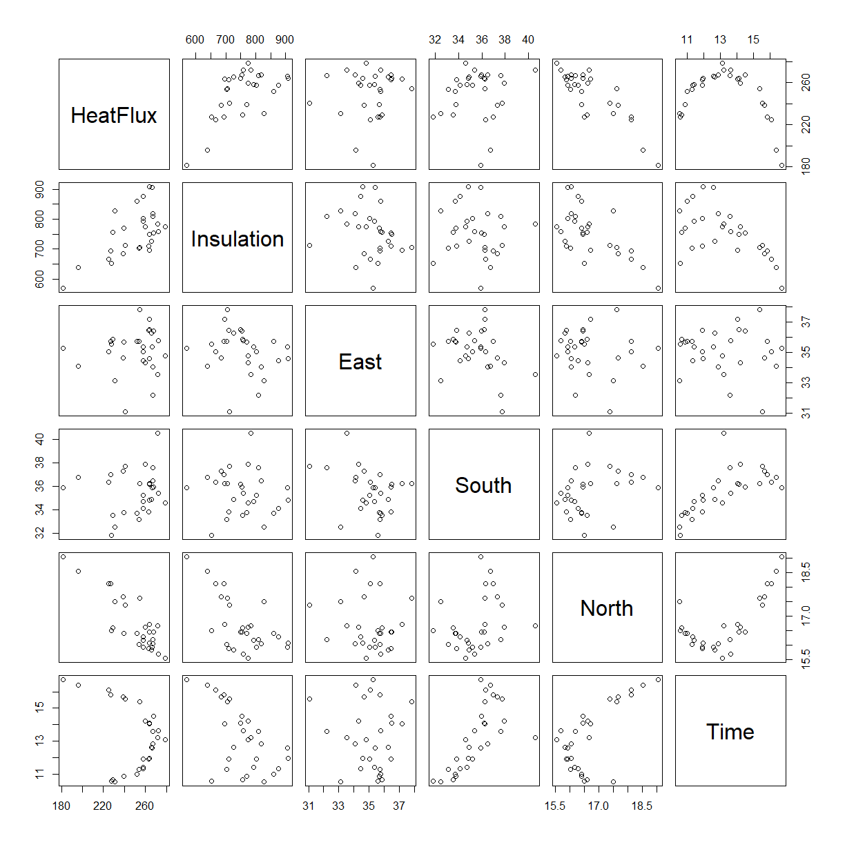
Note that HeatFlux appears to be approximately linearly related to all predictors except time. We will fit a multiple linear regression of HeatFlux ($Y$) on the predictors Insulation ($X_1$), East ($X_2$), South ($X_3$), North ($X_4$), and Time ($X_5$).
Suggested Model: $Y=\beta_0+\beta_1X_1+\beta_2X_2+\beta_3X_3+\beta_4X_4+\beta_5 X_5 + \varepsilon$
We will now fit this model in R and look at various outputs which I will intersperse with comments.
heatflux_fit <- lm(HeatFlux ~ Insulation + East + South + North + Time, data = heat_flux)

par(mfrow = c(2, 2))
plot(heatflux_fit)
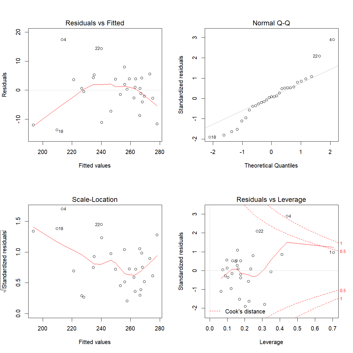
Looking at the Residual vs Fitted values plot, ignore the Loess smoother line fitted, if it wasn’t for a couple of points you probably would think this looks like a random scatter about zero so model adequate and proceed to check the normality assumption. The Normal Q-Q plot looks approximately linear so might be prepared to say the normality assumption holds. We are now in a position to make inference. Recall that you cannot test any hypotheses or obtain confidence intervals if the model assumptions do not hold.
summary(heatflux_fit)
Call:
lm(formula = HeatFlux ~ Insulation + East + South + North + Time,
    data = heat_flux)

Residuals:
     Min       1Q   Median       3Q      Max
-13.6848  -2.7688   0.6273   3.9166  17.3962

Coefficients:
             Estimate Std. Error t value Pr(>|t|)
(Intercept) 325.43612   96.12721   3.385  0.00255 **
Insulation    0.06753    0.02899   2.329  0.02900 *
East          2.55198    1.24824   2.044  0.05252 .
South         3.80019    1.46114   2.601  0.01598 *
North       -22.94947    2.70360  -8.488 1.53e-08 ***
Time          2.41748    1.80829   1.337  0.19433
---
Signif. codes:  0 '***' 0.001 '**' 0.01 '*' 0.05 '.' 0.1 ' ' 1

Residual standard error: 8.039 on 23 degrees of freedom
Multiple R-squared:  0.8988,	Adjusted R-squared:  0.8768
F-statistic: 40.84 on 5 and 23 DF,  p-value: 1.077e-10
The p-value for the F statistic is very small (much smaller than 0.05) so the regression is significant which means that at least one of the predictors is needed in the model. The five predictors explain for 87.7% of the variability in the response HeatFlux.
1.7.2 Multiple linear regression: matrix form
Model: $Y=\beta_0+\beta_1X_1+\cdots+\beta_pX_p+\varepsilon$
Matrix form: $y=X\beta+\varepsilon$, where $y=\left(\begin{matrix}y_1\\vdots\y_n\\end{matrix}\right)$, $X=\left(\begin{matrix}1&x_{11}&x_{12}&\cdots&x_{1p}\\vdots&\vdots&\vdots&&\vdots\1&x_{n1}&x_{n2}&\cdots&x_{np}\\end{matrix}\right)$, $\beta=\left(\begin{matrix}\beta_0\\beta_1\\vdots\\beta_p\\end{matrix}\right)$ and $\varepsilon=\left(\begin{matrix}\varepsilon_1\\vdots\\varepsilon_n\\end{matrix}\right) \sim N(\mathbf{0},\sigma^2\mathbf{I})$.
Matrix $X$ is called the data matrix or model matrix or the design matrix. The data matrix ($X$) displays the predictor data, one column for each predictor variable, together with a column of 1s (if there is an intercept in the model), and it shows the experimental design if the levels of the predictor variables are planned. Each row in the matrix $X$ shows the information on all predictors for one case.
The least squares estimates of the regression coefficients $\beta$ are those values $\hat{\beta}$ that minimise the ‘residual sum of squares’ function $SSE(\beta)=(y-X\beta)^T(y-X\beta)$.
Normal equations: $(X^TX)\hat{\beta}=X^Ty$
Solution: $\hat{\beta}=(X^TX)^{-1}X^Ty$ (provided the inverse exists).
The $(p+1)\times(p+1)$ matrix $(X^TX)$ is a symmetric matrix whose elements consist of sums of squares and sums of cross products of the elements in the columns of $X$. The nature of $(X^TX)$ plays an important role in the properties of the estimators $\hat{\beta}$ and will often be a large factor in the success or failure of the least squares estimation procedure.
Fitted values: $\hat{y}=X\hat{\beta}$
Residuals: $e=y-\hat{y}$.
Residual sum of squares: $SSE=(y-X\hat{\beta})^T(y-X\hat{\beta})=y^Ty-{\hat{\beta}}^T(X^TX)\hat{\beta}$
Unbiased estimate of $\sigma^2$: ${\hat{\sigma}}^2=\frac{1}{n-p-1}(y-X\hat{\beta})^T(y-X\hat{\beta})=\frac{1}{n-p-1}\sum{(y-{\hat{y}}_i)^2}$
Properties of the least squares estimators
$E(\hat{\beta})=E(X^TX)^{-1}X^Ty=\beta$.
$Var(\hat{\beta})=\sigma^2(X^TX)^{-1}$.
If we assume that $\varepsilon$ has a normal distribution, then $ \hat{\beta}$ also has a normal distribution with mean $\beta$ and variance $\sigma^2(X^TX)^{-1}$.
Here the distribution of the residual mean square is given by $\frac{(n-p-1)^2\hat{\sigma}^2}{\sigma^2} \sim \chi_{n-p-1}^2$. The estimated variance of $\hat{\beta}$ is given by $\hat{\sigma}^2(X^TX)^{-1}$, and standard errors are obtained as $\hat{\sigma}$ multiplied by the square root of the diagonal elements of the $(X^TX)^{-1}$ matrix.
Predictions and fitted values
If we observe a vector of predictors $x$ (including a 1) for which we don’t know the response, the predicted response is $\hat{y}=x^T\hat{\beta}$ with standard error of prediction $\mathrm{s.e.pred}=s\sqrt{1+x^T(X^TX)^{-1}x}$. Similarly, the estimated mean response when the predictors take the value $x$ is $\hat{y}=x^T\hat{\beta}$ with standard error of fit $\mathrm{s.e.}(\mathrm{fit})=s\sqrt{x^T(X^{T}X)^{-1}x}$.
2.1 HYPOTHESIS TESTS
We wish to test whether the overall regression is significant; i.e., are all the predictors taken together useful in the prediction of $Y$?
Should a particular predictor be in the regression model?
Should a set of predictors be added to the regression model? (This situation arises when a group of predictors belong together.)
In general, we have a null model (reduced model), in which some or all of the predictors are left out of the model (i.e. some or all of $\beta_i$’s are hypothesised to be zero) and a full model which has all the predictors in the model (i.e. all $\beta_i$’s present). The general form of the test statistic is:
where $\hat{\sigma}^2$ is the usual estimate of $\sigma^2$ under the full model and $\hat{\sigma}_0^2$ is the estimate of $\sigma^2$ under the null model (reduced model). If the null model holds $\hat{\sigma}_0^2$ equals $\sigma^2$ and if the null model does not hold then it is greater than $\sigma^2$. Having more parameters in the model will always reduce the residual variation. Therefore $\sigma^2\le\hat{\sigma}_0^2$.If the null model holds we would expect $F$ to be approximately equal to 1 and if the full model holds we would expect $F$ to be greater than 1. If $F$ is large the full model has reduced the residual variation substantially, the additional predictors are useful in the prediction of the $y$ whereas if $F$ is close to 1 then the additional predictors in the full model have not reduced the residual variation by much so we would use the null model.
2.1.1 Test for overall significance of the regression
If we had $p$ predictors the full model would be
If we are interested in testing whether the regression is significant or not we are interested in testing whether some of the predictors ($X_i$’s) are useful or not. The null model would be that none of the predictors are useful:
We test the hypothesis $H_0:\beta_1=\beta_2=\cdots=\beta_p=0$ against $H_1:$ at least one $\beta_i\neq0$. In matrix notation
Here the regression mean square would be used to estimate $\sigma^2$ under the full model and the residual mean square would be used to estimate $\sigma^2$ under the null model. The test statistic is
which under the null hypothesis has a $F_{p,n-p-1}$ distribution. We reject $H_0$ in favour of $H_1$ if $F$ lies in the upper tail of this distribution.
Computations can be summarised in the ANOVA table:
where $SST$, $SSR$ and $SSE$ are defined as before. We have exactly the same decomposition as before that
SST = SSR + SSE
Now, $R^2=\frac{SSR}{SST}$ is the proportion of the variance explained by the regression.
We can show that
A small value of $R^2$ will result in a small value of $F$ and we will not reject $H_0$ in favour of $H_1$. A value of $R^2$ close to 1 will result in a large value of $F$ and we will reject $H_0$ in favour of $H_1$.
We already have seen an example of testing whether the regression is significant.
2.1.2 Selecting the “best” model
There is no unique criterion for choosing the “best” model. We want as simple a model as possible that adequately explains what is going on (“principle of parsimony”). The more parameters in the model, the closer the fitted values will be to the observed data and the higher $R^2$ will be but the standard errors of the estimates ${\hat{\beta}}_i$ will increase because we are estimating more parameters on the same amount of information. We trade off between
- Few $X$’s (small $p$): lower $R^2$ but more precise $\beta_i$’s and
- Many $X$’s (large $p$): higher $R^2$ but less precise $\beta_i$’s.
We try to find that set of predictors which give an acceptable model fit, or $R^2$. If a predictor does not add to the model’s explanation of the variation of $Y$ in a significant way, it is not added to the model, even though it would have reduced $R^2$.
Comparing two models
The reduced model is the model with the smallest number of parameters. We want to test $H_0:$ reduced model is appropriate against $H_1:$ full model is appropriate. To formally test this we need to fit the reduced model and record from the output the Residual (Error) Sum of Squares and its associated degrees of freedom, which we denote by $SSE_{RM}$ and $DF_{RM}$ respectively. The same information is required from fitting the full model, label the residual sum of squares and its associated degrees of freedom by $SSE_{FM}$ and $DF_{FM}$. The appropriate test statistic is
We reject $H_0$ in favour of $H_1$ at the $100\alpha\%$ significance level if $T>F_{DF_{RM}-DF_{FM},DF_{FM};\alpha}$. This is only valid if the model assumptions hold. We will look at regression diagnostics in detail the next section.
Partial F-tests
Assume that we have $n$ observations. The full model has all the $p$ predictors in it. The reduced model has one predictor removed, say the i’th predictor. We use the same test statistic as above and reject $H_0:\beta_i=0$ in favour of $H_1:\beta_i\neq0$ at the $\alpha100\%$ significance level if $T>F_{1,n-p-1;\alpha}$. You can think of the partial F tests as assessing variables as if they were the last being added to the model.
An equivalent way of testing $H_0:\beta_i=0$ versus $H_1:\beta_i\neq 0$ is using
$t=\frac{\hat{\beta}i}{S.E.(\hat{\beta}}_i)}$
which has a $t{n-p-1}$ distribution if $H_0$ is true.
The R function lm gives you the partial F-tests in this way.
The disadvantage of partial F-tests is that they are not independent tests.
EXAMPLE: Heat Flux revisited
summary(heatflux_fit)
Call:
lm(formula = HeatFlux ~ Insulation + East + South + North + Time,
    data = heat_flux)

Residuals:
     Min       1Q   Median       3Q      Max
-13.6848  -2.7688   0.6273   3.9166  17.3962

Coefficients:
             Estimate Std. Error t value Pr(>|t|)
(Intercept) 325.43612   96.12721   3.385  0.00255 **
Insulation    0.06753    0.02899   2.329  0.02900 *
East          2.55198    1.24824   2.044  0.05252 .
South         3.80019    1.46114   2.601  0.01598 *
North       -22.94947    2.70360  -8.488 1.53e-08 ***
Time          2.41748    1.80829   1.337  0.19433
---
Signif. codes:  0 '***' 0.001 '**' 0.01 '*' 0.05 '.' 0.1 ' ' 1

Residual standard error: 8.039 on 23 degrees of freedom
Multiple R-squared:  0.8988,	Adjusted R-squared:  0.8768
F-statistic: 40.84 on 5 and 23 DF,  p-value: 1.077e-10
The Partial F-tests p-values are given in the Pr(>|t|) column. You only look at these if the
model assumptions hold. Suppose they do, then you would conclude at the 5% significance level
that the predictors Insulation and South are significant.
Sequential F tests
Assume that we have $Sn$ observations. Variables are added to the model in a particular order and at each step the most recent predictor being entered into the model is tested for significance.
R function lm can provide the output. All you need do is divide the sequential sum of squares
by the residual mean sum of squares for the full model and compare with $F_{1,n-p-1}$.
The advantage of the sequential $F$ tests are that they are independent tests.
The disadvantage is that the tests may be highly dependent on the order in which the
predictors enter the model.
fit5 <- lm(HeatFlux ~ Insulation + East + South + North + Time, data = heat_flux)
fit4 <- lm(HeatFlux ~ Insulation + East + South + North, data = heat_flux)
fit3 <- lm(HeatFlux ~ Insulation + East + South, data = heat_flux)
fit2 <- lm(HeatFlux ~ Insulation + East, data = heat_flux)
fit1 <- lm(HeatFlux ~ Insulation, data = heat_flux)
fit0 <- lm(HeatFlux ~ 1, data = heat_flux)

anova(fit0, fit1, fit2, fit3, fit4, fit5, test = "F")
Analysis of Variance Table

Model 1: HeatFlux ~ 1
Model 2: HeatFlux ~ Insulation
Model 3: HeatFlux ~ Insulation + East
Model 4: HeatFlux ~ Insulation + East + South
Model 5: HeatFlux ~ Insulation + East + South + North
Model 6: HeatFlux ~ Insulation + East + South + North + Time
  Res.Df     RSS Df Sum of Sq       F    Pr(>F)
1     28 14681.9
2     27  8898.1  1    5783.8 89.4964 2.155e-09 ***
3     26  8086.4  1     811.7 12.5602 0.0017316 **
4     25  6904.9  1    1181.5 18.2822 0.0002832 ***
5     24  1601.9  1    5303.0 82.0574 4.772e-09 ***
6     23  1486.4  1     115.5  1.7873 0.1943335
---
Signif. codes:  0 '***' 0.001 '**' 0.01 '*' 0.05 '.' 0.1 ' ' 1
East, South and North are significant (at 1\% significance level or 0.5\% significance level) according to the Sequential F Test.
EXERCISE Try different orderings of the predictors. There are 5 ways you can choose the first predictor, 4 ways for the second predictor, 3 ways of choosing the third predictor, 2 ways of choosing the fourth predictor, and only one way to choose the fifth predictor giving $5 \times 4 \times 3 \times 2 \times 1 = 120$ combinations.
Using R Square ($R^2$)
When a linear regression model is fitted using function lm in R you can extract $R^2$.
summary(heatflux_fit)$r.squared
[1] 0.8987602
R Square gives the “proportion of variation in the response data that is explained by the model”. An acceptable value for $R^2$ depends on the context of the model fitting. R Square ($R^2$) is a dangerous criterion for model comparisons, any additional model terms will automatically increase it.
Note that Multiple R-squared given earlier is the same as R-squared in the lm function.
Using Adjusted R Square ($R_{ADJ}^2$)
When a linear regression model is fitted using lm in R you can always obtain $R_{ADJ}^2$
(Adjusted R-Squared). This is $R_{ADJ}^2=1-\frac{n-1}{n-p}(1-R^2)$ which does not necessarily
increase if more terms are added to the model. The model with the largest $R_{ADJ}^2$ is usually
chosen.
EXAMPLE For the Heat Flux data using all the predictors the Adjusted R-squared is 0.8768. See earlier output.
Using $\hat{\sigma}^2$, the residual mean square (MSE)
We choose the model with the smallest $\hat{\sigma}^2$ or if the next smallest $\hat{\sigma}^2$ is close to the smallest $\hat{\sigma}^2$ but the model has less terms in it we would choose it.
Mallows $C_p$ (A Criterion Based Method)
Predicted values obtained from a regression equation based on a subset of variables are generally biased. We use the mean square error of the predicted value to judge the performance of an equation. The measure standardized total mean squared error of prediction for the observed data by
where MSE($\hat{y}_i$) is the ith predicted value from an equation with $p$ terms (number of parameters in equation) and $\sigma^2$ is the variance of the random errors. This statistic places special emphasis on observed data, and good subsets will result in small values.
We can estimate the value of this statistic from the data by Mallows’ $C$, calculated from:
where $\hat{\sigma}^2$ is from the linear model with the full set of $q$ variables.
Mallows’ $C_p$ has these properties:
- it is easily calculated from usual regression summaries,
- it measures the difference in fitting errors between the full and the subset models,
- it has a random and a fixed component giving a trade off between better fit and more parameters, and
- it can be used to compare subset models — although it is not necessarily true that a smaller value means a better subset model, any model with $C_p \le p$ will be a good model.
We can use leaps to obtain the Mallow’s $C_p$. Note that when $p$ equals the number of
predictors in the full model that Mallow’s $C_p$ always equals $p$.
library(leaps)

x <- heat_flux[, -1]
y <- heat_flux$HeatFlux

leaps(x, y)
$which
      1     2     3     4     5
1 FALSE FALSE FALSE  TRUE FALSE
1  TRUE FALSE FALSE FALSE FALSE
1 FALSE FALSE FALSE FALSE  TRUE
1 FALSE FALSE  TRUE FALSE FALSE
1 FALSE  TRUE FALSE FALSE FALSE
2 FALSE FALSE  TRUE  TRUE FALSE
2 FALSE FALSE FALSE  TRUE  TRUE
2  TRUE FALSE FALSE  TRUE FALSE
2 FALSE  TRUE FALSE  TRUE FALSE
2  TRUE  TRUE FALSE FALSE FALSE
2  TRUE FALSE  TRUE FALSE FALSE
2  TRUE FALSE FALSE FALSE  TRUE
2 FALSE FALSE  TRUE FALSE  TRUE
2 FALSE  TRUE FALSE FALSE  TRUE
2 FALSE  TRUE  TRUE FALSE FALSE
3 FALSE  TRUE  TRUE  TRUE FALSE
3  TRUE FALSE  TRUE  TRUE FALSE
3 FALSE FALSE  TRUE  TRUE  TRUE
3  TRUE FALSE FALSE  TRUE  TRUE
3 FALSE  TRUE FALSE  TRUE  TRUE
3  TRUE  TRUE FALSE  TRUE FALSE
3  TRUE  TRUE  TRUE FALSE FALSE
3  TRUE FALSE  TRUE FALSE  TRUE
3 FALSE  TRUE  TRUE FALSE  TRUE
3  TRUE  TRUE FALSE FALSE  TRUE
4  TRUE  TRUE  TRUE  TRUE FALSE
4  TRUE FALSE  TRUE  TRUE  TRUE
4 FALSE  TRUE  TRUE  TRUE  TRUE
4  TRUE  TRUE FALSE  TRUE  TRUE
4  TRUE  TRUE  TRUE FALSE  TRUE
5  TRUE  TRUE  TRUE  TRUE  TRUE

$label
[1] "(Intercept)" "1"           "2"           "3"           "4"
[6] "5"

$size
 [1] 2 2 2 2 2 3 3 3 3 3 3 3 3 3 3 4 4 4 4 4 4 4 4 4 4 5 5 5 5 5 6

$Cp
 [1]  38.492277 112.687090 174.174842 199.329010 199.803490   9.097518
 [7]  17.846129  37.462451  40.490491 102.126871 107.320539 114.607262
[13] 120.046927 174.732260 196.395794   7.596312   9.717698   9.950942
[19]  10.149946  19.842738  38.941581  85.844637 100.383642 101.484104
[25] 102.842597   5.787266   8.179844   9.424426  10.764344  76.054147
[31]   6.000000
According to Mallow’s $C_p$ none of the models are any good.
Multicollinearity
When predictors are related to each other, regression modelling can be very confusing. Estimated effects can change in magnitude and even sign. Two predictors are collinear if $c_1x_1+c_2x_2=c_0$ for constants $c_1,c_2,c_0$. The definition of collinearity extends to several predictors. More important, however, is approximate collinearity, when predictors are closely but not exactly related and the equation holds approximately. In some packages (e.g. Minitab) a message is given if you perform a regression where there is too much collinearity. If the collinearity is extreme, a variable will be dropped before the calculations are carried out. If the collinearity is exact, this causes no loss of information, and if the collinearity is approximate, only a small amount of information is lost.
Alternatively, we can ask for variance inflation factors (VIFs) associated with each predictor. These come from the formula for the variance of the parameter estimates $Var(\hat{\beta}_i)=\sigma^2\left(\frac{1}{1-R_i^2}\right)\left(\frac{1}{SX_iX_i}\right)$, with $R_i^2$ the square of the multiple correlation between $X_i$ and the other $X’s$, and $1/(1-R_i^2)$ being the amount by which the variance is increased, or inflated, due to collinearity. If none of the VIFs are greater than 10 then collinearity is not a problem.
EXAMPLE Revisiting Heat Flux example.
library(car)

heatflux_fit <- lm(HeatFlux ~ Insulation + East + South + North + Time, data = heat_flux)
vif(heatflux_fit)
Insulation       East      South      North       Time
  2.319035   1.355448   3.175970   2.612066   5.370059
All VIFs are less than 10 so there is no multicollinearity problem.
Multiple correlation coefficient
The multiple correlation coefficient $R_{Y|X_1,\cdots,X_p}$ is a measure of the association between $Y$ and $X_1,\ldots,X_p$ jointly. Its square is what we have called $R^2$. We can interpret $R_{Y|X_1,\cdots,X_p}$ as the correlation between $Y$ and the regression equation involving $X_1,\ldots,X_p$. It is defined as $R_{Y|X_1,\cdots,X_p}=\frac{\sum(y_i-\bar{y})(y_i-\hat{y})}{\sum(y_i-\bar{y})^2 \sum (y_i-\bar\hat{y})^2}$ where $\hat{y}i=\hat{\beta}_0+\hat{\beta}_1x{i1}+\hat{\beta}2x{i2}+\cdots \hat{\beta}px{ip}$, $i=1,\ldots,n$, is the fitted value or predicted value for $y_i$ and $\bar\hat{y}=\frac{1}{n}\sum \hat{y}_i$ is the mean of the fitted values. (It turns out that $\bar{\hat{y}}=\bar{y}$ always.)
Also, $R_{Y|X_1,\cdots,X_p}^2=\frac{SST-SSE}{SST}=\frac{SSR}{SST}$ and it is interpreted as the proportion of total variation (SST) that is explained by the regression involving $X_1,\ldots,X_p$ (SSR).
Variable selection
To combat collinearity or to find a parsimonious model we may wish to select only some of the predictor variables available. Assume that we have $n$ cases with values observed on $k$ predictor variables $X_1,X_2,\cdots,X_k$ and a response $Y$. Let $p$ = the number of predictors in a selected subset (including the intercept) and assume all necessary transformations have been carried out.
The full model can be written as $Y=X_1\beta_1+X_2\beta_2+\varepsilon$ (vector notation, with X_1 an n by p matrix) and the subset model $Y=X_1\beta_1+\varepsilon$ is obtained by putting $\beta_2=0$. The subset model is tested against the full model using a generalised F-test, as usual.
Selecting variables on substantive grounds
The most important method for selecting variables is based on a knowledge of the situation and the variables being studied.
EXAMPLE: The variables HT (height) and WT (weight) can be combined into
BMI (body mass index = weight per height squared).
EXAMPLE: A number of test scores can be combined into an average.
EXAMPLE: Weisberg (1981) gives an example Highway data, from a Masters thesis modelling the automobile accident rate in terms of 13 independent variables. Here there are $2^{13} = 8192$ possible subset models, which can be reduced by considering two points:
- Three variables,
FAI,PAandMA, should be kept together since they are indicator variables for different types of highways, with a fourth type indicated if each of these variables equals zero and - The variable
LEN, length of segment under study, is required by definition. This now gives a total of 512 possible subset models, still a large number but much fewer than originally.
Stepwise methods of variable selection
Often we have to use the data to find a reasonable subset of the predictors for use in a model. A stepwise procedure is a systematic way of examining only a few subsets of each size and choosing a path through all possible models.
Forward selection
We begin with a simple regression model with the best single predictor (largest $R^2$, $F$ or $t$).We then add the predictor that increases $R^2$ the most, or would have the largest $F$ or $t$ of any of the other variables. We continue thus, but stop when you reach a subset of predetermined size, or when no other variable has an $F$ greater than $F$ to enter, or if any variable would cause unacceptable collinearity.
Backward elimination
We begin with the full model. We then remove the variable with the smallest $F$ or $t$, the variable that would reduce $R^2$ the least. We continue thus, but stop when you reach a subset of predetermined size, or when all variables remaining in the model have $F$ greater than $F$ to remove.
Stepwise
This is a combination of the previous two methods. We start with one variable, as in forward selection, and at each step take one of four options: add a variable, remove a variable, exchange two variables or stop. If there are at least two variables in the model, remove a variable if it has $F$ less than $F$ to remove. If there are at least two variables in the model, remove a variable if this would result in a larger $R^2$ than obtained previously with that many variables. Exchange a variable in the model with one not in the model if this would increase $R^2$. Add a variable if it has the largest $F$ greater than $F$ to enter and the collinearity tolerance is OK.
Remarks
- Stepwise methods entail less computing than Best Subsets Regression.
- Order in which variables enter or leave the equation should not be interpreted as reflecting the relative importance of the variables.
- If data is noncollinear, all three methods should give nearly the same selection of variables.
- CHP recommend Backward Elimination over Forward Selection because the full variable set is calculated and available for inspection even though it may not be used in the final equation.
- Backward Elimination copes better with multicollinearity.
- Residual plots for various “best” models fitted to data should always be examined and if found to be unsatisfactory the model should not be used.
EXAMPLE: Squid data (This data set is from Classical and Modern Regression with Applications by R.H. Myers published in 1990.) An experiment was conducted to study the size of squid eaten by sharks and tuna.
The regressors are characteristics of the beak or mouth of the squid. They are X1 = Beak length in inches, X2 = Wing length in inches, X3 = Beak to notch length, X4 = Notch to wing length, and X5 = Width in inches. The response (Y) is the weight of the squid in pounds. These data are given below.
We first fit the model $Y=\beta_0+\beta_1X_1+\beta_2X_2+\beta_3X_3+\beta_4X_4+\beta_5X_5+\varepsilon$ to the above data.
Before doing this we should first obtain a matrix scatter plot of the data.
library(tidyverse)
library(ggpubr)

squid <- read_csv(file.path("..", "Data", "Squid.csv"))
squid
# A tibble: 22 x 6
       Y    X1    X2    X3    X4    X5
   <dbl> <dbl> <dbl> <dbl> <dbl> <dbl>
 1  1.95  1.31  1.07  0.44 0.75  0.35
 2  2.9   1.55  1.49  0.53 0.9   0.47
 3  0.72  0.99  0.84  0.34 0.570 0.32
 4  0.81  0.99  0.83  0.34 0.54  0.27
 5  1.09  1.05  0.9   0.36 0.64  0.3
 6  1.22  1.09  0.93  0.42 0.61  0.31
 7  1.02  1.08  0.9   0.4  0.51  0.31
 8  1.93  1.27  1.08  0.44 0.77  0.34
 9  0.64  0.99  0.85  0.36 0.56  0.290
10  2.08  1.34  1.13  0.45 0.77  0.37
# ... with 12 more rows
pairs(squid)
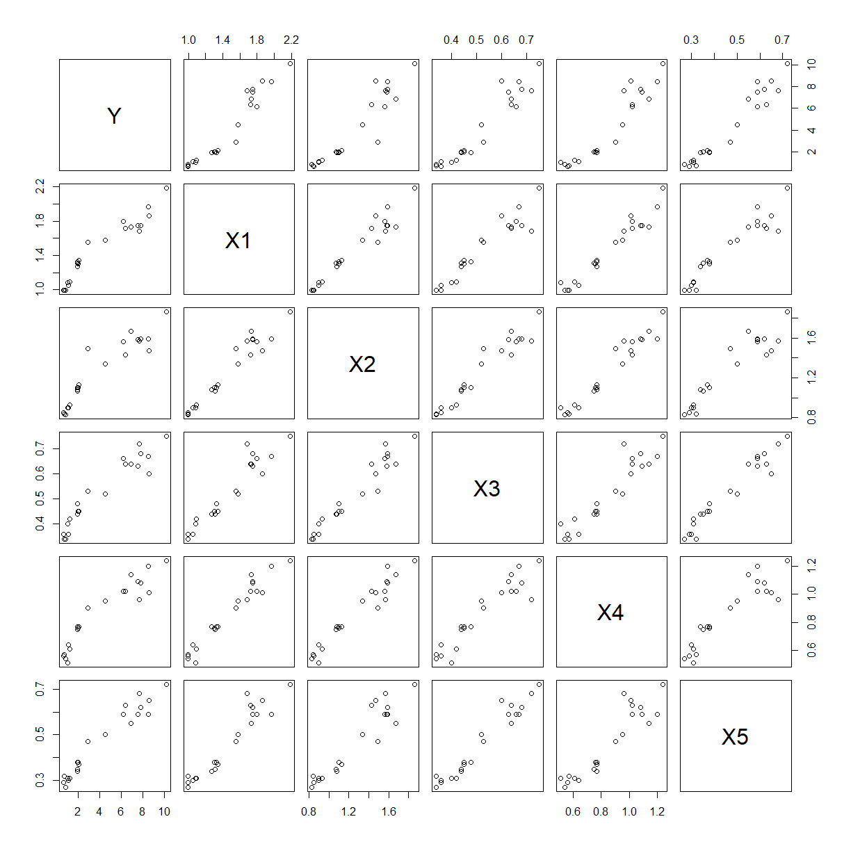
The relationship between $Y$ and each predictor separately is approximately linear with positive slope. More worrying is the obvious correlations between most of the predictors, there may be multicollinearity.
Seeing what happens when we fit the multiple linear regression.
squid_fit <- lm(Y ~ X1 + X2 + X3 + X4 + X5, data = squid)

par(mfrow = c(2, 2))
plot(squid_fit)
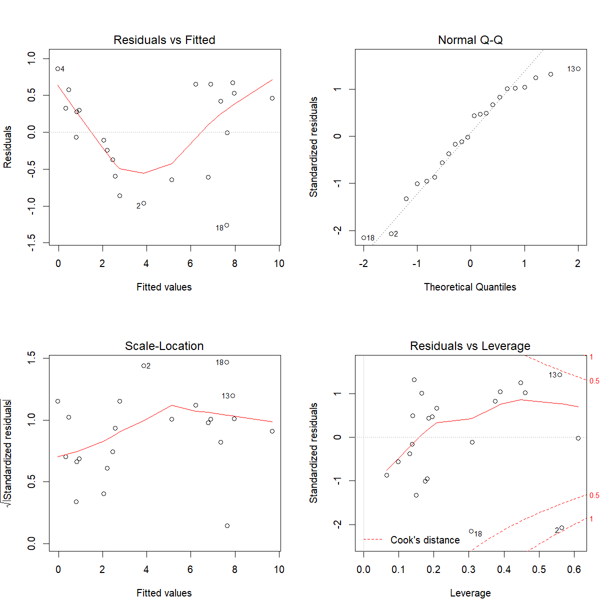
The model is not adequate, the Residual versus Fitted values plot does not look like a random scatter about zero. We cannot proceed to make valid inference.
For the moment, just to illustrate what to do if the model was adequate and the normality assumption held, look at the model out put.
summary(squid_fit)
Call:
lm(formula = Y ~ X1 + X2 + X3 + X4 + X5, data = squid)

Residuals:
    Min      1Q  Median      3Q     Max
-1.2610 -0.5373  0.1355  0.5120  0.8611

Coefficients:
            Estimate Std. Error t value Pr(>|t|)
(Intercept)  -6.5122     0.9336  -6.976 3.13e-06 ***
X1            1.9994     2.5733   0.777  0.44851
X2           -3.6751     2.7737  -1.325  0.20378
X3            2.5245     6.3475   0.398  0.69610
X4            5.1581     3.6603   1.409  0.17791
X5           14.4012     4.8560   2.966  0.00911 **
---
Signif. codes:  0 '***' 0.001 '**' 0.01 '*' 0.05 '.' 0.1 ' ' 1

Residual standard error: 0.7035 on 16 degrees of freedom
Multiple R-squared:  0.9633,	Adjusted R-squared:  0.9519
F-statistic: 84.07 on 5 and 16 DF,  p-value: 6.575e-11
Partial F tests suggest that the “best” model contains only one predictor variable and that is X5. (Since the model assumptions are violated the above inference is dangerous.)
We could also look at the “best” model suggested by sequential F tests. The order in which the parameters are listed can affect the conclusions reached significantly. A full-scale model-building process cannot be based on sequential F tests unless there is an appropriate selection of order of variables based on subject matter expertise.
fit5 <- lm(Y ~ X1 + X2 + X3 + X4 + X5, data = squid)
fit4 <- lm(Y ~ X1 + X2 + X3 + X4, data = squid)
fit3 <- lm(Y ~ X1 + X2 + X3, data = squid)
fit2 <- lm(Y ~ X1 + X2, data = squid)
fit1 <- lm(Y ~ X1, data = squid)
fit0 <- lm(Y ~ 1, data = squid)

anova(fit0, fit1, fit2, fit3, fit4, fit5, test = "F")
Analysis of Variance Table

Model 1: Y ~ 1
Model 2: Y ~ X1
Model 3: Y ~ X1 + X2
Model 4: Y ~ X1 + X2 + X3
Model 5: Y ~ X1 + X2 + X3 + X4
Model 6: Y ~ X1 + X2 + X3 + X4 + X5
  Res.Df     RSS Df Sum of Sq        F    Pr(>F)
1     21 215.925
2     20  16.779  1   199.145 402.4397 9.131e-13 ***
3     19  16.653  1     0.127   0.2560  0.619804
4     18  12.533  1     4.120   8.3249  0.010765 *
5     17  12.270  1     0.263   0.5325  0.476114
6     16   7.918  1     4.352   8.7951  0.009109 **
---
Signif. codes:  0 '***' 0.001 '**' 0.01 '*' 0.05 '.' 0.1 ' ' 1
The model suggested by the sequential F tests is $Y=\beta_0+\beta_1X_1+\beta_3X_3+\beta_5X_5+\varepsilon$.
fit135 <- lm(Y ~ X1 + X3 + X5, data = squid)

summary(fit135)
Call:
lm(formula = Y ~ X1 + X3 + X5, data = squid)

Residuals:
    Min      1Q  Median      3Q     Max
-1.6386 -0.5084  0.1060  0.5471  0.9666

Coefficients:
            Estimate Std. Error t value Pr(>|t|)
(Intercept) -6.83999    0.87718  -7.798 3.52e-07 ***
X1           3.26593    1.60373   2.036   0.0567 .
X3           0.07094    5.48254   0.013   0.9898
X5          13.35925    4.72866   2.825   0.0112 *
---
Signif. codes:  0 '***' 0.001 '**' 0.01 '*' 0.05 '.' 0.1 ' ' 1

Residual standard error: 0.7142 on 18 degrees of freedom
Multiple R-squared:  0.9575,	Adjusted R-squared:  0.9504
F-statistic: 135.1 on 3 and 18 DF,  p-value: 1.572e-12
The appropriate test statistic for testing $H_0: Y=\beta_0+\beta_1X_1+\beta_3X_3+\beta_5X_5+\varepsilon$ against $H_1: Y=\beta_0+\beta_1X_1+\beta_2X_2+\beta_3X_3+\beta_4X_4+\beta_5X_5+\varepsilon$ is
We reject $H_0$ in favour of $H_1$ at the 100$\alpha\%$ significance level if $T>F_{DF_{RM}-DF_{FM},DF_{FM};\alpha}$.
anova(fit5)
Analysis of Variance Table

Response: Y
          Df  Sum Sq Mean Sq  F value    Pr(>F)
X1         1 199.145 199.145 402.4397 9.131e-13 ***
X2         1   0.127   0.127   0.2560  0.619804
X3         1   4.120   4.120   8.3249  0.010765 *
X4         1   0.263   0.263   0.5325  0.476114
X5         1   4.352   4.352   8.7951  0.009109 **
Residuals 16   7.918   0.495
---
Signif. codes:  0 '***' 0.001 '**' 0.01 '*' 0.05 '.' 0.1 ' ' 1
anova(fit135)
Analysis of Variance Table

Response: Y
          Df  Sum Sq Mean Sq  F value    Pr(>F)
X1         1 199.145 199.145 390.3744 1.188e-13 ***
X3         1   3.525   3.525   6.9103   0.01704 *
X5         1   4.072   4.072   7.9816   0.01121 *
Residuals 18   9.183   0.510
---
Signif. codes:  0 '***' 0.001 '**' 0.01 '*' 0.05 '.' 0.1 ' ' 1
Now, from the output above $SSE_{FM}=7.918$, $DF_{FM}=16$, $SSE_{REM}=9.183$, and $DF_{RM}=18$ so our test statistic
Need to compare this with $F_{2,18;0.05}$.
qf(0.95, df1 = 2, df2 = 18)
[1] 3.554557
Since $T=1.28 \ngeq 3.5546$ we cannot reject $H_0$ in favour of $H_1$ at the $5\%$ significance level. The reduced model here is plausible.
If the model assumptions were not being met the above inference is dangerous.
Forward stepwise regression in R
Illustrated on the squid data set.
model <- lm(Y ~ ., data = squid)
model$call$data <- squid # Should not be needed when running by hand

ols_step_forward_p(model)
Forward Selection Method
---------------------------

Candidate Terms:

1. X1
2. X2
3. X3
4. X4
5. X5

We are selecting variables based on p value...

Variables Entered:

- X5
- X4
- X2

No more variables to be added.

Final Model Output
------------------

                        Model Summary
--------------------------------------------------------------
R                       0.981       RMSE                0.678
R-Squared               0.962       Coef. Var          16.169
Adj. R-Squared          0.955       MSE                 0.460
Pred R-Squared          0.930       MAE                 0.524
--------------------------------------------------------------
 RMSE: Root Mean Square Error
 MSE: Mean Square Error
 MAE: Mean Absolute Error

                               ANOVA
--------------------------------------------------------------------
               Sum of
              Squares        DF    Mean Square       F         Sig.
--------------------------------------------------------------------
Regression    207.643         3         69.214     150.44    0.0000
Residual        8.281        18          0.460
Total         215.925        21
--------------------------------------------------------------------

                                  Parameter Estimates
----------------------------------------------------------------------------------------
      model      Beta    Std. Error    Std. Beta      t        Sig      lower     upper
----------------------------------------------------------------------------------------
(Intercept)    -5.980         0.659                 -9.073    0.000    -7.365    -4.596
         X5    17.109         3.082        0.798     5.551    0.000    10.634    23.584
         X4     6.879         2.783        0.489     2.472    0.024     1.033    12.726
         X2    -2.890         2.346       -0.292    -1.232    0.234    -7.820     2.040
----------------------------------------------------------------------------------------
                           Selection Summary
-----------------------------------------------------------------------
        Variable                  Adj.
Step    Entered     R-Square    R-Square     C(p)       AIC       RMSE
-----------------------------------------------------------------------
   1    X5            0.9455      0.9428    5.7794    54.6672    0.7670
   2    X4            0.9584      0.9540    2.1456    50.7185    0.6875
   3    X2            0.9616      0.9553    2.7354    50.9387    0.6783
-----------------------------------------------------------------------
Final model has $X_5$, $X_4$ and $X_2$.
Forward stepwise elimination in R
modelb <- lm(Y ~ ., data = squid)
modelb$call$data <- squid # Should not be needed when running by hand

ols_step_backward_p(modelb)
Backward Elimination Method
---------------------------

Candidate Terms:

1 . X1
2 . X2
3 . X3
4 . X4
5 . X5

We are eliminating variables based on p value...

Variables Removed:

- X3
- X1

No more variables satisfy the condition of p value = 0.3


Final Model Output
------------------

                        Model Summary
--------------------------------------------------------------
R                       0.981       RMSE                0.678
R-Squared               0.962       Coef. Var          16.169
Adj. R-Squared          0.955       MSE                 0.460
Pred R-Squared          0.930       MAE                 0.524
--------------------------------------------------------------
 RMSE: Root Mean Square Error
 MSE: Mean Square Error
 MAE: Mean Absolute Error

                               ANOVA
--------------------------------------------------------------------
               Sum of
              Squares        DF    Mean Square       F         Sig.
--------------------------------------------------------------------
Regression    207.643         3         69.214     150.44    0.0000
Residual        8.281        18          0.460
Total         215.925        21
--------------------------------------------------------------------

                                  Parameter Estimates
----------------------------------------------------------------------------------------
      model      Beta    Std. Error    Std. Beta      t        Sig      lower     upper
----------------------------------------------------------------------------------------
(Intercept)    -5.980         0.659                 -9.073    0.000    -7.365    -4.596
         X2    -2.890         2.346       -0.292    -1.232    0.234    -7.820     2.040
         X4     6.879         2.783        0.489     2.472    0.024     1.033    12.726
         X5    17.109         3.082        0.798     5.551    0.000    10.634    23.584
----------------------------------------------------------------------------------------
                          Elimination Summary
-----------------------------------------------------------------------
        Variable                  Adj.
Step    Removed     R-Square    R-Square     C(p)       AIC       RMSE
-----------------------------------------------------------------------
   1    X3             0.963      0.9543    4.1582    52.1665    0.6858
   2    X1            0.9616      0.9553    2.7354    50.9387    0.6783
-----------------------------------------------------------------------
Final model has $X_2$, $X_4$ and $X_5$.
Stepwise regression in R
models <- lm(Y ~ ., data = squid)
models$call$data <- squid # Should not be needed when running by hand

ols_step_both_p(models)
Stepwise Selection Method
---------------------------

Candidate Terms:

1. X1
2. X2
3. X3
4. X4
5. X5

We are selecting variables based on p value...

Variables Entered/Removed:

- X5 added
- X4 added

No more variables to be added/removed.


Final Model Output
------------------

                        Model Summary
--------------------------------------------------------------
R                       0.979       RMSE                0.687
R-Squared               0.958       Coef. Var          16.387
Adj. R-Squared          0.954       MSE                 0.473
Pred R-Squared          0.945       MAE                 0.529
--------------------------------------------------------------
 RMSE: Root Mean Square Error
 MSE: Mean Square Error
 MAE: Mean Absolute Error

                               ANOVA
--------------------------------------------------------------------
               Sum of
              Squares        DF    Mean Square       F         Sig.
--------------------------------------------------------------------
Regression    206.945         2        103.473    218.947    0.0000
Residual        8.979        19          0.473
Total         215.925        21
--------------------------------------------------------------------

                                   Parameter Estimates
-----------------------------------------------------------------------------------------
      model      Beta    Std. Error    Std. Beta       t        Sig      lower     upper
-----------------------------------------------------------------------------------------
(Intercept)    -6.335         0.601                 -10.543    0.000    -7.593    -5.077
         X5    15.016         2.606        0.700      5.763    0.000     9.562    20.470
         X4     4.154         1.710        0.295      2.429    0.025     0.574     7.734
-----------------------------------------------------------------------------------------
                            Stepwise Selection Summary
-----------------------------------------------------------------------------------
                     Added/                   Adj.
Step    Variable    Removed     R-Square    R-Square     C(p)       AIC       RMSE
-----------------------------------------------------------------------------------
   1       X5       addition       0.946       0.943    5.7790    54.6672    0.7670
   2       X4       addition       0.958       0.954    2.1460    50.7185    0.6875
-----------------------------------------------------------------------------------
Final model has $X_5$ and $X_4$.
Best Subsets Regression in R
modelbs <- lm(Y ~ ., data = squid)
modelbs$call$data <- squid # Should not be needed when running by hand

ols_step_best_subset(modelbs)
   Best Subsets Regression
-----------------------------
Model Index    Predictors
-----------------------------
     1         X5
     2         X4 X5
     3         X2 X4 X5
     4         X1 X2 X4 X5
     5         X1 X2 X3 X4 X5
-----------------------------

                                                 Subsets Regression Summary
-----------------------------------------------------------------------------------------------------------------------------
                       Adj.        Pred
Model    R-Square    R-Square    R-Square     C(p)       AIC        SBIC        SBC       MSEP      FPE       HSP       APC
-----------------------------------------------------------------------------------------------------------------------------
  1        0.9455      0.9428      0.9343    5.7794    54.6672     -8.0766    57.9403    0.6475    0.6418    0.0310    0.0654
  2        0.9584      0.9540      0.9448    2.1456    50.7185    -10.5305    55.0827    0.5490    0.5370    0.0263    0.0547
  3        0.9616      0.9553      0.9301    2.7354    50.9387     -9.1759    56.3940    0.5659    0.5437    0.0271    0.0554
  4        0.9630      0.9543      0.9262    4.1582    52.1665     -6.9128    58.7128    0.6147    0.5772    0.0294    0.0588
  5        0.9633      0.9519        0.91    6.0000    53.9501     -4.2645    61.5874    0.6898    0.6298    0.0330    0.0642
-----------------------------------------------------------------------------------------------------------------------------
AIC: Akaike Information Criteria
 SBIC: Sawa's Bayesian Information Criteria
 SBC: Schwarz Bayesian Criteria
 MSEP: Estimated error of prediction, assuming multivariate normality
 FPE: Final Prediction Error
 HSP: Hocking's Sp
 APC: Amemiya Prediction Criteria
Using Mallow’s $C_p$ would go for Model 3. Full model always has Mallow’s $C_p = p$.
Using Adjusted $R^2$ would go for Model 3.
Other packages will give you the estimate of $\hat{\sigma}^2$ or $\hat{\sigma}$ for each model and you would go for the model with the smallest or close to smallest $\hat{\sigma}^2$ with the least number of parameters in it.
2.2 PARTIAL CORRELATION
Partial correlation is the correlation between two variables while controlling for the effects
of one or more other variables.The partial correlation between $Y$ and $X$, after controlling
for $Z_1,\cdots,Z_p$ is denoted by $r_{YX|Z_1,cdots,Z_p}$. Its square is defined as follows
$r_{YX|Z_1,\cdots,Z_p}^2=\frac{SSE_{Z_1,\cdots,Z_p}-SSE_{X,Z_1,\cdots,Z_p}}{SSE_{Z_1,\cdots,Z_p}}$.
This is the reduction in sum of squares due to adding $X$ into the model, given $Z_1,\cdots,Z_p$
already in the model divided by the residual sum of squares for the model only having
$Z_1,\cdots,Z_p$. The quantity $r_{YX|Z_1,\cdots,Z_p}$ is called the $p^{th}$ order partial
correlation coefficient. The R package ppcor can be used to calculate partial correlations.
See https://cran.r-project.org/web/packages/ppcor/ppcor.pdf. If we compare the controlled
correlation ($r_{YX|Z_1,\cdots,Z_p}$) with the original correlation ($r_{YX}$) and if there is
no difference, the inference is that the control variables have no effect.
Test of the partial correlation coefficient
The partial correlation coefficient is an estimate $r_{YX|Z_1,\cdots,Z_p}^2$ of the population quantity $\rho_{YX|Z_1,\ldots,Z_p}^2$. We test $H_0:\rho_{YX|Z_1,\ldots,Z_p}^2=0$ versus $H_1:\rho_{YX|Z_1,\ldots,Z_p}^2\neq0$ via the partial F-test with test statistic $T=\frac{\left(SSE_{RM}-SSE_{FM}\right)/(DF_{RM}-DF_{FM})}{SSE_{FM}/DF_{FM}}$ where the reduced model regresses $Y$ on $Z_1,\cdots,Z_p$ and the full model regresses $Y$ on $X,Z_1,\cdots,Z_p$.
EXAMPLE: MCG (For details see http://www.statsci.org/data/oz/afl.html)
Want to investigate the effect on football game attendance of various covariates.
After taking the effect of Members into account, what is the effect of Top50 on MCG attendance? Here $Y=$MCG, $X=$Top50 and $Z=$Members.
library(tidyverse)

mcg1 <- read_csv(file.path("..", "Data", "MCG1.csv"))
mcg1
# A tibble: 41 x 8
     MCG Other  Temp Members Top50 Date       Home  Away
   <dbl> <dbl> <dbl>   <dbl> <dbl> <chr>      <chr> <chr>
 1  8.65 72.9     24    12.6     5 27/03/1993 NM    Bris
 2 49.9  60.8     21    26.0     7 3/04/1993  Ess   Carl
 3 24.4  59.8     24    16.9     5 17/04/1993 NM    Melb
 4 46.6   9.27    22    27.0     8 1/05/1993  Ess   Gee
 5 29.3  74.8     17    22.9     7 8/05/1993  Rich  StK
 6 34.4  61.9     16    51.6     8 22/05/1993 Ess   Adel
 7 17.8  92.1     19    13.0     4 29/05/1993 Rich  Syd
 8 37.1  23.4     13    29.9     9 12/06/1993 Carl  Gee
 9 44.1  61.2     14    21.6     6 19/06/1993 Melb  Ess
10 19.1  54.9     13    21.5     7 26/06/1993 Ess   Rich
# ... with 31 more rows
Fitting the model without the controlling variable.
mcg_fit1 <- lm(MCG ~ Members, data = mcg1)

summary(mcg_fit1)
Call:
lm(formula = MCG ~ Members, data = mcg1)

Residuals:
    Min      1Q  Median      3Q     Max
-37.602  -8.161  -0.114   8.453  31.575

Coefficients:
            Estimate Std. Error t value Pr(>|t|)
(Intercept)   9.6216     8.0103   1.201 0.236935
Members       1.2073     0.2873   4.202 0.000149 ***
---
Signif. codes:  0 '***' 0.001 '**' 0.01 '*' 0.05 '.' 0.1 ' ' 1

Residual standard error: 15.57 on 39 degrees of freedom
Multiple R-squared:  0.3117,	Adjusted R-squared:  0.294
F-statistic: 17.66 on 1 and 39 DF,  p-value: 0.0001488
anova(mcg_fit1)
Analysis of Variance Table

Response: MCG
          Df Sum Sq Mean Sq F value    Pr(>F)
Members    1 4279.8  4279.8   17.66 0.0001488 ***
Residuals 39 9451.5   242.3
---
Signif. codes:  0 '***' 0.001 '**' 0.01 '*' 0.05 '.' 0.1 ' ' 1
Fitting the model with the controlling variable.
mcg_fit2 <- lm(MCG ~ Members + Top50, data = mcg1)

summary(mcg_fit2)
Call:
lm(formula = MCG ~ Members + Top50, data = mcg1)

Residuals:
    Min      1Q  Median      3Q     Max
-38.124  -9.259   0.387   8.682  30.940

Coefficients:
            Estimate Std. Error t value Pr(>|t|)
(Intercept)   1.5101    11.1320   0.136  0.89281
Members       1.0728     0.3143   3.413  0.00154 **
Top50         1.9474     1.8584   1.048  0.30130
---
Signif. codes:  0 '***' 0.001 '**' 0.01 '*' 0.05 '.' 0.1 ' ' 1

Residual standard error: 15.55 on 38 degrees of freedom
Multiple R-squared:  0.331,	Adjusted R-squared:  0.2958
F-statistic: 9.401 on 2 and 38 DF,  p-value: 0.0004818
anova(mcg_fit2)
Analysis of Variance Table

Response: MCG
          Df Sum Sq Mean Sq F value    Pr(>F)
Members    1 4279.8  4279.8 17.7044 0.0001518 ***
Top50      1  265.5   265.5  1.0981 0.3012961
Residuals 38 9186.0   241.7
---
Signif. codes:  0 '***' 0.001 '**' 0.01 '*' 0.05 '.' 0.1 ' ' 1
Calculating the partial correlation:
cor(mcg1$MCG, mcg1$Top50)
[1] 0.3548781
Now correlation between MCG and Top50 is 0.355. After controlling for Members, the correlation between MCG and Top50 has shrunk to 0.17.
3.1 CONFOUNDING
An extraneous variable is an independent variable that is not of direct interest to the study, but does have an influence on the response.
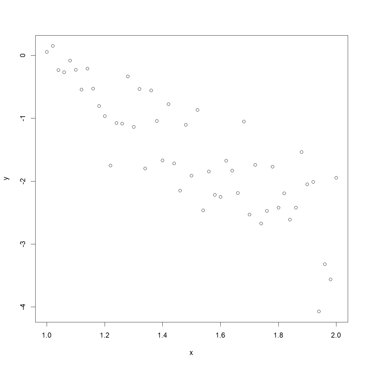
EXAMPLE: We observe the following relationship between characteristics $y$ and $x$ in a sample of male members of a species:
males <- read_csv(file.path("..", "Data", "Males.csv"))

plot(males)
and the following for the females:
females <- read_csv(file.path("..", "Data", "Females.csv"))

plot(females)
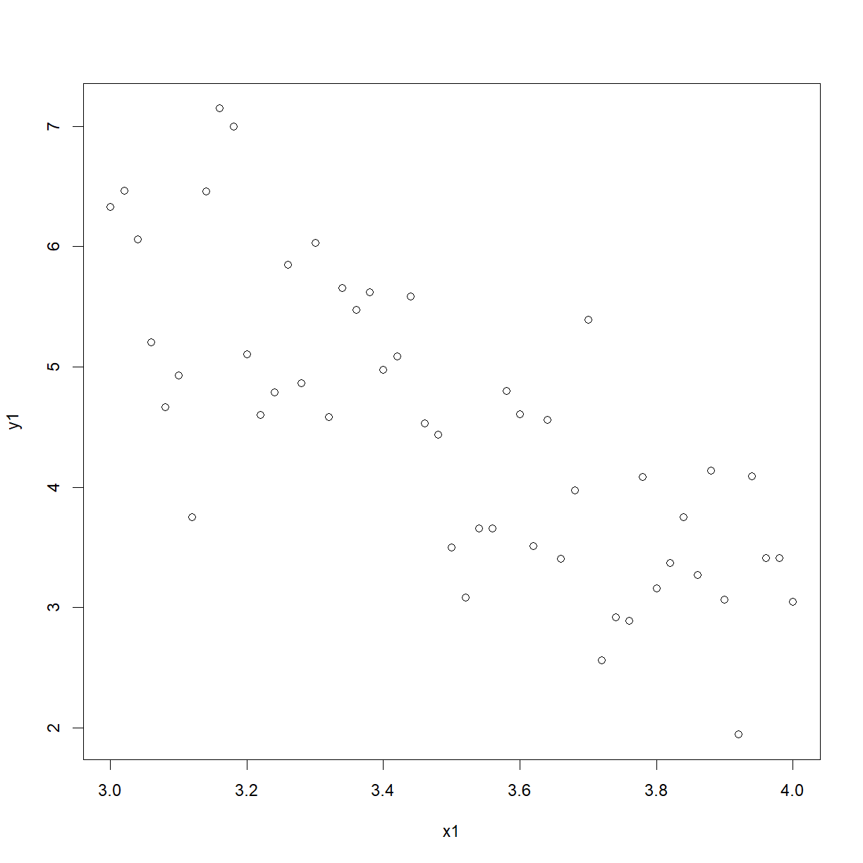
Plots look very similar but the ranges on the x-axes and y- axes are different.
Simple linear regression for the genders separately give:
Males
males_fit <- lm(y ~ x, data = males)

summary(males_fit)
Call:
lm(formula = y ~ x, data = males)

Residuals:
     Min       1Q   Median       3Q      Max
-1.33527 -0.36645  0.03395  0.36717  1.03367

Coefficients:
            Estimate Std. Error t value Pr(>|t|)
(Intercept)   2.5815     0.3820   6.758 1.57e-08 ***
x            -2.7407     0.2499 -10.967 8.60e-15 ***
---
Signif. codes:  0 '***' 0.001 '**' 0.01 '*' 0.05 '.' 0.1 ' ' 1

Residual standard error: 0.5254 on 49 degrees of freedom
Multiple R-squared:  0.7105,	Adjusted R-squared:  0.7046
F-statistic: 120.3 on 1 and 49 DF,  p-value: 8.599e-15
anova(males_fit)
Analysis of Variance Table

Response: y
          Df Sum Sq Mean Sq F value    Pr(>F)
x          1 33.199  33.199  120.28 8.599e-15 ***
Residuals 49 13.525   0.276
---
Signif. codes:  0 '***' 0.001 '**' 0.01 '*' 0.05 '.' 0.1 ' ' 1
plot(males)
abline(a = 2.5815, b = -2.7407)
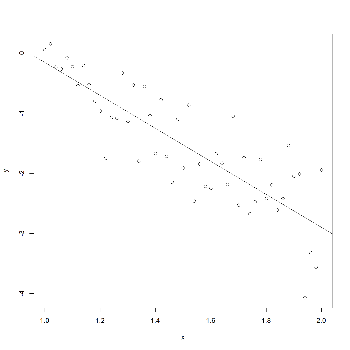
Females
females_fit <- lm(y1 ~ ., data = females)

summary(females_fit)
Call:
lm(formula = y1 ~ ., data = females)

Residuals:
     Min       1Q   Median       3Q      Max
-1.90342 -0.61669  0.05136  0.53750  1.61836

Coefficients:
            Estimate Std. Error t value Pr(>|t|)
(Intercept)  15.3054     1.3308  11.501 1.59e-15 ***
x1           -3.0930     0.3789  -8.163 1.08e-10 ***
---
Signif. codes:  0 '***' 0.001 '**' 0.01 '*' 0.05 '.' 0.1 ' ' 1

Residual standard error: 0.7966 on 49 degrees of freedom
Multiple R-squared:  0.5763,	Adjusted R-squared:  0.5676
F-statistic: 66.64 on 1 and 49 DF,  p-value: 1.077e-10
anova(females_fit)
Analysis of Variance Table

Response: y1
          Df Sum Sq Mean Sq F value    Pr(>F)
x1         1 42.286  42.286  66.637 1.077e-10 ***
Residuals 49 31.094   0.635
---
Signif. codes:  0 '***' 0.001 '**' 0.01 '*' 0.05 '.' 0.1 ' ' 1
plot(females)
abline(a = 15.3054, b = -3.0930)
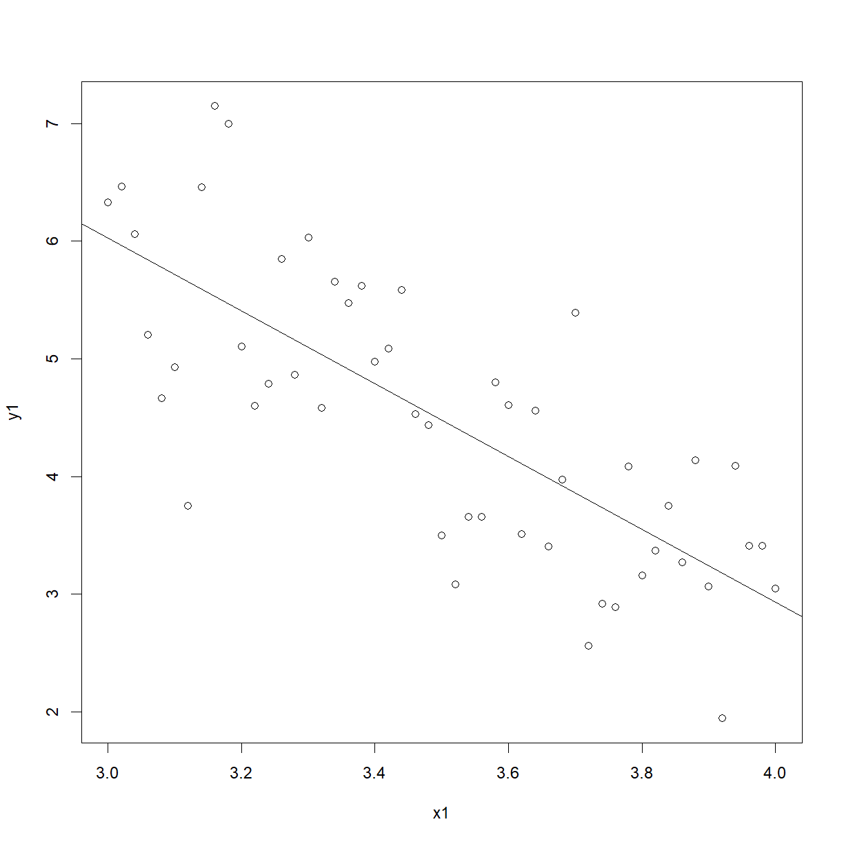
Intercepts ($\hat{\beta}_0$’s) are quite different for male and female regression equations but slopes ($\hat{\beta}_1’s$) are similar.
Reasonable to conclude that there is a negative linear relationship between Y and X, with a slope of -3. (Test $H_0:\beta_1=-3$ against $H_1:\beta_1\neq-3$ for Males and Females separately to see this.)
EXERCISE: Do this for yourself.
Now we regress $Y$ on $X$ with the males and females together:
mf <- read_csv(file.path("..", "Data", "MF.csv"))
mf
# A tibble: 102 x 3
       x       y   Sex
   <dbl>   <dbl> <dbl>
 1  1     0.0573     1
 2  1.02  0.151      1
 3  1.04 -0.235      1
 4  1.06 -0.265      1
 5  1.08 -0.0827     1
 6  1.1  -0.227      1
 7  1.12 -0.544      1
 8  1.14 -0.208      1
 9  1.16 -0.530      1
10  1.18 -0.803      1
# ... with 92 more rows
mf_fit <- lm(y ~ x, data = mf)
summary(mf_fit)
Call:
lm(formula = y ~ x, data = mf)

Residuals:
    Min      1Q  Median      3Q     Max
-4.1277 -1.4482 -0.1652  1.4083  4.0033

Coefficients:
            Estimate Std. Error t value Pr(>|t|)
(Intercept)  -4.8558     0.4675  -10.39   <2e-16 ***
x             2.5324     0.1726   14.67   <2e-16 ***
---
Signif. codes:  0 '***' 0.001 '**' 0.01 '*' 0.05 '.' 0.1 ' ' 1

Residual standard error: 1.817 on 100 degrees of freedom
Multiple R-squared:  0.6828,	Adjusted R-squared:  0.6797
F-statistic: 215.3 on 1 and 100 DF,  p-value: < 2.2e-16
Overall regression has a slope of $\hat{\beta}_1=2.5324$! This is what has happened:
plot(mf$x, mf$y)
abline(a = -4.8558, b = 2.5324)
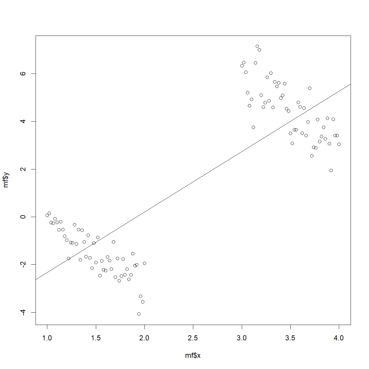
Plot of $y$ vs $x$, with genders indicated by different symbols:
ggplot(mf, aes(x = x, y = y, colour = Sex)) +
    geom_point() +
    geom_abline(intercept = -4.8558, slope = 2.5324)
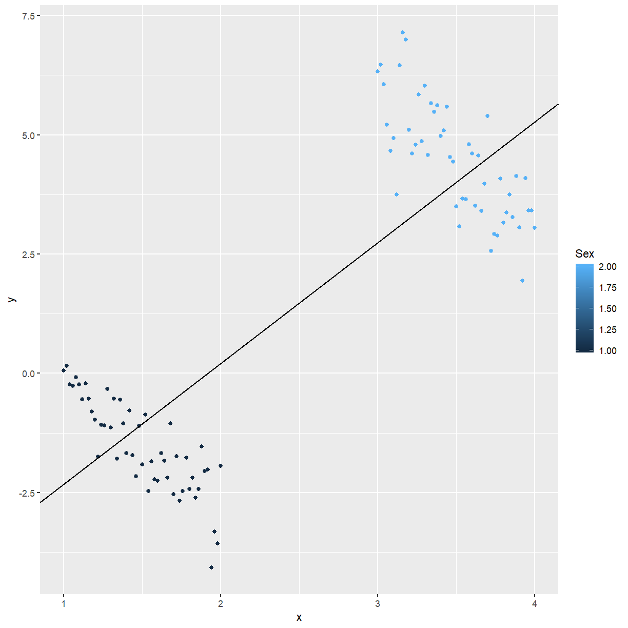
Gender is a confounder in the regression. A confounder is a variable in a study that may not be of direct interest, but has an association with both response and predictor(s). Confounders must be taken into account or controlled for. If not, incorrect results such as that shown above may be obtained.
Kleinbaum et al [1] state: In general, confounding exists if meaningfully different interpretations of the relationship of interest result when an extraneous variable is ignored or included in the data analysis.
[1] Kleinbaum, Kupper, Muller and Nizam (1998) Applied Regression Analysis and Other Multivariable Methods, Third Edition, Duxbury Press.
Controlling for a confounder
mf_fit_all <- lm(y ~ ., data = mf)

summary(mf_fit_all)
Call:
lm(formula = y ~ ., data = mf)

Residuals:
    Min      1Q  Median      3Q     Max
-1.8365 -0.4415 -0.0187  0.4624  1.6783

Coefficients:
            Estimate Std. Error t value Pr(>|t|)
(Intercept)  -8.9972     0.2393  -37.59   <2e-16 ***
x            -2.9168     0.2265  -12.88   <2e-16 ***
Sex          11.8430     0.4722   25.08   <2e-16 ***
---
Signif. codes:  0 '***' 0.001 '**' 0.01 '*' 0.05 '.' 0.1 ' ' 1

Residual standard error: 0.6734 on 99 degrees of freedom
Multiple R-squared:  0.9569,	Adjusted R-squared:  0.956
F-statistic:  1098 on 2 and 99 DF,  p-value: < 2.2e-16
anova(mf_fit_all)
Analysis of Variance Table

Response: y
          Df Sum Sq Mean Sq F value    Pr(>F)
x          1 710.81  710.81 1567.49 < 2.2e-16 ***
Sex        1 285.24  285.24  629.03 < 2.2e-16 ***
Residuals 99  44.89    0.45
---
Signif. codes:  0 '***' 0.001 '**' 0.01 '*' 0.05 '.' 0.1 ' ' 1
FIXME To put a plot with the fitted model here
How do we identify when confounding is occurring?
The coefficient of a predictor is very different when the confounder is added to the model.
EXAMPLE: When the model is $Y_i=\beta_0+\beta_1X_i+\varepsilon$ for above example we get $\hat{\beta}_1=2.5324$. When gender is added to the model:
we get $\hat{\beta}_1=-2.9168$. This is ample proof of confounding. No formal statistical test for the equality of the $\beta_1$’s obtained under the two models exists; we need to use judgement, in conjunction with graphical evidence such as above. Confounding happens when both response and predictor are affected by the same variable. Evidence of the cause of confounding is provided by plots of both $X$ and $Y$ against the confounder.
par(mfrow = c(1, 2))
boxplot(x ~ Sex, data = mf)
boxplot(y ~ Sex, data = mf)
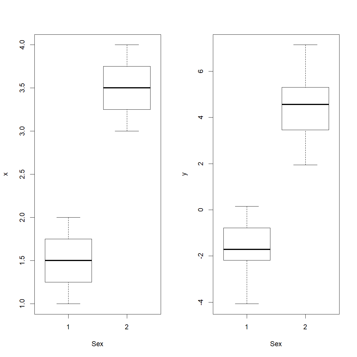
Continuous confounders
EXAMPLE: Mass and Physical Measurements for Male Subjects Michael Larner measured the weight and various physical measurements for 22 male subjects aged 16 - 30. Subjects were randomly chosen volunteers, all in reasonable good health. Subjects were requested to slightly tense each muscle being measured to ensure measurement consistency. All measurements except mass are in cm.
Larner, M. (1996). Mass and its Relationship to Physical Measurements. MS305 Data Project, Department of Mathematics, University of Queensland.
Say the purpose of the study was to explain men’s weight ($Y$) as a function of their height ($X_1$):
mass <- read_csv(file.path("..", "Data", "mass.csv"))
names(mass) <- c("Mass", "Fore", "Bicep", "Chest", "Neck", "Shoulder", "Waist", "Height",
    "Calf", "Thigh", "Head")
mass
# A tibble: 22 x 11
    Mass  Fore Bicep Chest  Neck Shoulder Waist Height  Calf Thigh  Head
   <dbl> <dbl> <dbl> <dbl> <dbl>    <dbl> <dbl>  <dbl> <dbl> <dbl> <dbl>
 1  77    28.5  33.5   100  38.5      114  85     178   37.5  53    58
 2  85.5  29.5  36.5   107  39        119  90.5   187   40    52    59
 3  63    25    31      94  36.5      102  80.5   175   33    49    57
 4  80.5  28.5  34     104  39        114  91.5   183   38    50    60
 5  79.5  28.5  36.5   107  39        114  92     174   40    53    59
 6  94    30.5  38     112  39        121 101     180   39.5  57.5  59
 7  66    26.5  29      93  35        105  76     178.  38.5  50    58.5
 8  69    27    31      95  37        108  84     182.  36    49    60
 9  65    26.5  29      93  35        112  74     178.  34    47    55.5
10  58    26.5  31      96  35        103  76     168.  35    46    58
# ... with 12 more rows
mass_fit1 <- lm(Mass ~ Height, data = mass)

summary(mass_fit1)
Call:
lm(formula = Mass ~ Height, data = mass)

Residuals:
     Min       1Q   Median       3Q      Max
-14.2156  -7.7434   0.1785   4.0739  18.7436

Coefficients:
            Estimate Std. Error t value Pr(>|t|)
(Intercept) -81.3253    61.4763  -1.323    0.201
Height        0.8699     0.3443   2.527    0.020 *
---
Signif. codes:  0 '***' 0.001 '**' 0.01 '*' 0.05 '.' 0.1 ' ' 1

Residual standard error: 9.781 on 20 degrees of freedom
Multiple R-squared:  0.242,	Adjusted R-squared:  0.2041
F-statistic: 6.385 on 1 and 20 DF,  p-value: 0.02004
anova(mass_fit1)
Analysis of Variance Table

Response: Mass
          Df  Sum Sq Mean Sq F value  Pr(>F)
Height     1  610.86  610.86  6.3854 0.02004 *
Residuals 20 1913.29   95.66
---
Signif. codes:  0 '***' 0.001 '**' 0.01 '*' 0.05 '.' 0.1 ' ' 1
An extraneous variable in the study is $X_2=$ Waist. Let’s add it into the regression:
mass_fit2 <- lm(Mass ~ Height + Waist, data = mass)

summary(mass_fit2)
Call:
lm(formula = Mass ~ Height + Waist, data = mass)

Residuals:
    Min      1Q  Median      3Q     Max
-8.9319 -3.2881  0.6235  3.5401  5.2012

Coefficients:
            Estimate Std. Error t value Pr(>|t|)
(Intercept) -89.3517    26.0808  -3.426  0.00283 **
Height        0.3439     0.1559   2.206  0.03990 *
Waist         1.1909     0.1240   9.604    1e-08 ***
---
Signif. codes:  0 '***' 0.001 '**' 0.01 '*' 0.05 '.' 0.1 ' ' 1

Residual standard error: 4.147 on 19 degrees of freedom
Multiple R-squared:  0.8705,	Adjusted R-squared:  0.8569
F-statistic: 63.88 on 2 and 19 DF,  p-value: 3.678e-09
anova(mass_fit2)
Analysis of Variance Table

Response: Mass
          Df  Sum Sq Mean Sq F value    Pr(>F)
Height     1  610.86  610.86  35.514 9.788e-06 ***
Waist      1 1586.49 1586.49  92.237 1.005e-08 ***
Residuals 19  326.80   17.20
---
Signif. codes:  0 '***' 0.001 '**' 0.01 '*' 0.05 '.' 0.1 ' ' 1
We have
The estimate of $\beta_1$ differs substantially depending on whether Waist is included in the model or not. Confounding is occurring because of important association between the extraneous variable (Waist) and the response variable Mass.
It is often necessary to include in a model variables not of direct interest to the research question (i.e. extraneous variables), simply because omitting them from the analysis would lead to incorrect conclusions concerning the relationship between the variables of interest.
How do we know what extraneous variables, or potential confounders, to measure in a study?
We have to rely on previous knowledge, such as that gained from previous studies, to identify which variables, besides those of direct interest, we should be measuring.
3.2 Interaction
Interaction occurs when the relationship between $Y$ and $X_1$ is different at different levels of a third variable $X_2$.
EXAMPLE: Simulated data set. There is a continuous predictor $x_1$, and a categorical predictor $x_2$ which assumes the values 0 and 1. The variable $y$ increases linearly with $x_1$ when $x_2=0$, and decreases linearly with $x_1$ when $x_2=1$.
confounding <- read_csv(file.path("..", "Data", "confounding.csv"))
names(confounding) <- c("y", "x1", "x2")

ggplot(confounding, aes(x = x1, y = y, colour = x2)) +
    ggtitle("Figure 1: Interaction") +
    geom_point()
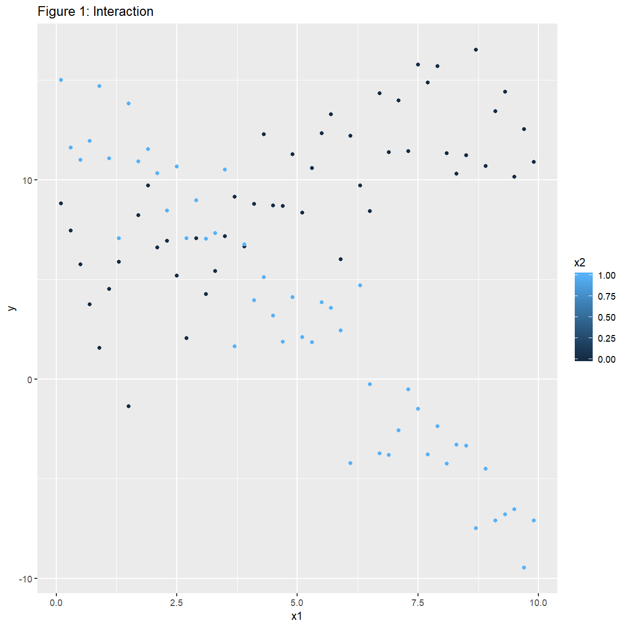
An example of no interaction is:
noconfounding <- read_csv(file.path("..", "Data", "noconfounding.csv"))
names(noconfounding) <- c("y", "x1", "x2")

ggplot(noconfounding, aes(x = x1, y = y, colour = x2)) +
    ggtitle("Figure 2: No interaction") +
    geom_point()
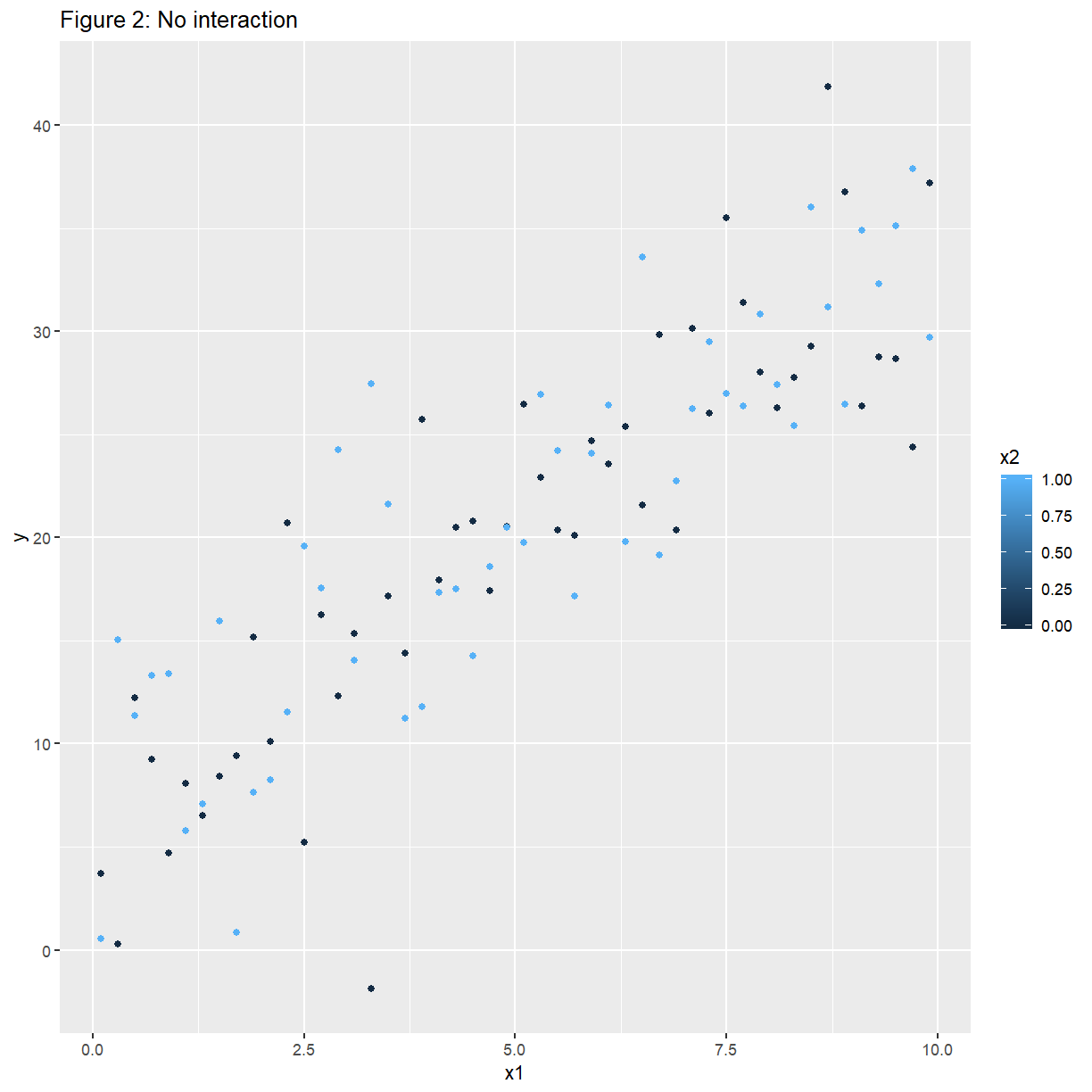
Here $y$ increases linearly with $x_1$, at the same rate (slope), irrespective of the value of $x_2$.
A regression of $Y$ on $X_1$ and $X_2$ for the data in Figure 1 gives:
conf_fit <- lm(y ~ x1 + x2, data = confounding)

summary(conf_fit)
Call:
lm(formula = y ~ x1 + x2, data = confounding)

Residuals:
     Min       1Q   Median       3Q      Max
-12.8407  -4.2836   0.0165   4.0220   9.5455

Coefficients:
            Estimate Std. Error t value Pr(>|t|)
(Intercept)  12.4042     1.1830  10.485  < 2e-16 ***
x1           -0.6230     0.1833  -3.399 0.000982 ***
x2           -6.2591     1.0580  -5.916 4.96e-08 ***
---
Signif. codes:  0 '***' 0.001 '**' 0.01 '*' 0.05 '.' 0.1 ' ' 1

Residual standard error: 5.29 on 97 degrees of freedom
Multiple R-squared:  0.3243,	Adjusted R-squared:  0.3104
F-statistic: 23.28 on 2 and 97 DF,  p-value: 5.539e-09
anova(conf_fit)
Analysis of Variance Table

Response: y
          Df  Sum Sq Mean Sq F value    Pr(>F)
x1         1  323.32  323.32  11.554 0.0009825 ***
x2         1  979.39  979.39  34.999 4.956e-08 ***
Residuals 97 2714.43   27.98
---
Signif. codes:  0 '***' 0.001 '**' 0.01 '*' 0.05 '.' 0.1 ' ' 1
We are fitting a common slope, and allowing different intercepts for $x_2=0$ and $x_2=1$. We can write the model as
ggplot(confounding, aes(x = x1, y = y, colour = x2)) +
    geom_point() +
    geom_abline(intercept = 12.4, slope = -0.623) +
    geom_abline(intercept = 6.14, slope = -0.623)
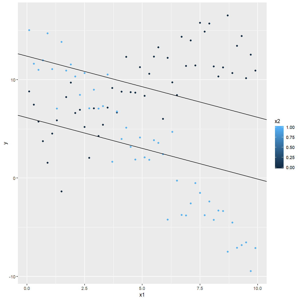
In order to capture the true relationship, we include an interaction term, which is $x_1\times x_2:$
conf_fit_int <- lm(y ~ x1 * x2, data = confounding)

summary(conf_fit_int)
Call:
lm(formula = y ~ x1 * x2, data = confounding)

Residuals:
    Min      1Q  Median      3Q     Max
-7.1629 -1.3032  0.0645  1.4364  4.5780

Coefficients:
            Estimate Std. Error t value Pr(>|t|)
(Intercept)   4.2929     0.6598   6.507 3.48e-09 ***
x1            0.9992     0.1143   8.743 7.42e-14 ***
x2            9.9634     0.9331  10.678  < 2e-16 ***
x1:x2        -3.2445     0.1616 -20.074  < 2e-16 ***
---
Signif. codes:  0 '***' 0.001 '**' 0.01 '*' 0.05 '.' 0.1 ' ' 1

Residual standard error: 2.332 on 96 degrees of freedom
Multiple R-squared:   0.87,	Adjusted R-squared:  0.8659
F-statistic: 214.2 on 3 and 96 DF,  p-value: < 2.2e-16
anova(conf_fit_int)
Analysis of Variance Table

Response: y
          Df  Sum Sq Mean Sq F value    Pr(>F)
x1         1  323.32  323.32  59.435 1.165e-11 ***
x2         1  979.39  979.39 180.039 < 2.2e-16 ***
x1:x2      1 2192.20 2192.20 402.985 < 2.2e-16 ***
Residuals 96  522.23    5.44
---
Signif. codes:  0 '***' 0.001 '**' 0.01 '*' 0.05 '.' 0.1 ' ' 1
We now have the following model:
The fitted lines are shown with the data below:
ggplot(confounding, aes(x = x1, y = y, colour = x2)) +
    geom_point() +
    geom_abline(intercept =  4.29, slope =  0.999) +
    geom_abline(intercept = 14.25, slope = -2.241)
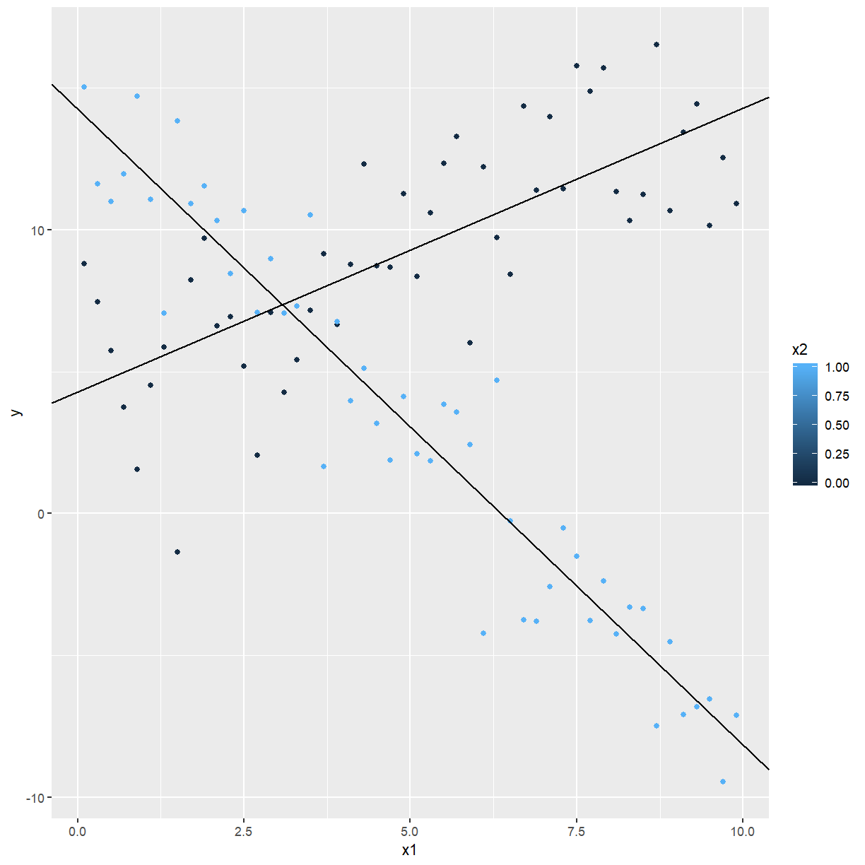
Fitting a model with an interaction term to the data in Figure 2 gives:
noconf_fit_int <- lm(y ~ x1 * x2, data = noconfounding)

summary(noconf_fit_int)
Call:
lm(formula = y ~ x1 * x2, data = noconfounding)

Residuals:
     Min       1Q   Median       3Q      Max
-16.8783  -3.0603  -0.4352   3.0126  11.3395

Coefficients:
            Estimate Std. Error t value Pr(>|t|)
(Intercept)   5.1814     1.3786   3.758 0.000294 ***
x1            2.9798     0.2388  12.479  < 2e-16 ***
x2            2.0335     1.9496   1.043 0.299551
x1:x2        -0.2760     0.3377  -0.817 0.415830
---
Signif. codes:  0 '***' 0.001 '**' 0.01 '*' 0.05 '.' 0.1 ' ' 1

Residual standard error: 4.873 on 96 degrees of freedom
Multiple R-squared:  0.7476,	Adjusted R-squared:  0.7397
F-statistic: 94.79 on 3 and 96 DF,  p-value: < 2.2e-16
anova(noconf_fit_int)
Analysis of Variance Table

Response: y
          Df Sum Sq Mean Sq  F value Pr(>F)
x1         1 6727.3  6727.3 283.2649 <2e-16 ***
x2         1   10.7    10.7   0.4498 0.5041
x1:x2      1   15.9    15.9   0.6678 0.4158
Residuals 96 2279.9    23.7
---
Signif. codes:  0 '***' 0.001 '**' 0.01 '*' 0.05 '.' 0.1 ' ' 1
The interaction term $x_1x_2$ is not significant. Fitting a model without the interaction term gives:
noconf_fit <- lm(y ~ x1 + x2, data = noconfounding)

summary(noconf_fit)
Call:
lm(formula = y ~ x1 + x2, data = noconfounding)

Residuals:
     Min       1Q   Median       3Q      Max
-17.1129  -3.0653  -0.6238   3.2418  11.5741

Coefficients:
            Estimate Std. Error t value Pr(>|t|)
(Intercept)   5.8713     1.0880   5.397 4.81e-07 ***
x1            2.8418     0.1686  16.859  < 2e-16 ***
x2            0.6537     0.9730   0.672    0.503
---
Signif. codes:  0 '***' 0.001 '**' 0.01 '*' 0.05 '.' 0.1 ' ' 1

Residual standard error: 4.865 on 97 degrees of freedom
Multiple R-squared:  0.7459,	Adjusted R-squared:  0.7406
F-statistic: 142.3 on 2 and 97 DF,  p-value: < 2.2e-16
anova(noconf_fit)
Analysis of Variance Table

Response: y
          Df Sum Sq Mean Sq  F value Pr(>F)
x1         1 6727.3  6727.3 284.2383 <2e-16 ***
x2         1   10.7    10.7   0.4513 0.5033
Residuals 97 2295.8    23.7
---
Signif. codes:  0 '***' 0.001 '**' 0.01 '*' 0.05 '.' 0.1 ' ' 1
Some comments in fitting a model with interaction
In general, an $m$’th order interaction involves $m+1$ predictors.
EXAMPLE: If we have the second-order $X_1X_2X_3$ interaction, we would also include the first-order interactions $X_1X_2$, $X_1X_3$ and $X_2X_3$ as well as the main effects $X_1$, $X_2$ and $X_3$.
-
When fitting a higher-order interaction term, we always include the corresponding lower-order terms in the model.
-
A model with interaction terms is more difficult to interpret than one with just main effects.
-
The higher the order of the interactions, the harder the interpretation becomes.
-
We will always prefer a model with fewer interaction terms if the models have similar $R_{Adj}^2$.
Some other diagnostics
par(mfrow = c(2, 2))
plot(noconf_fit)
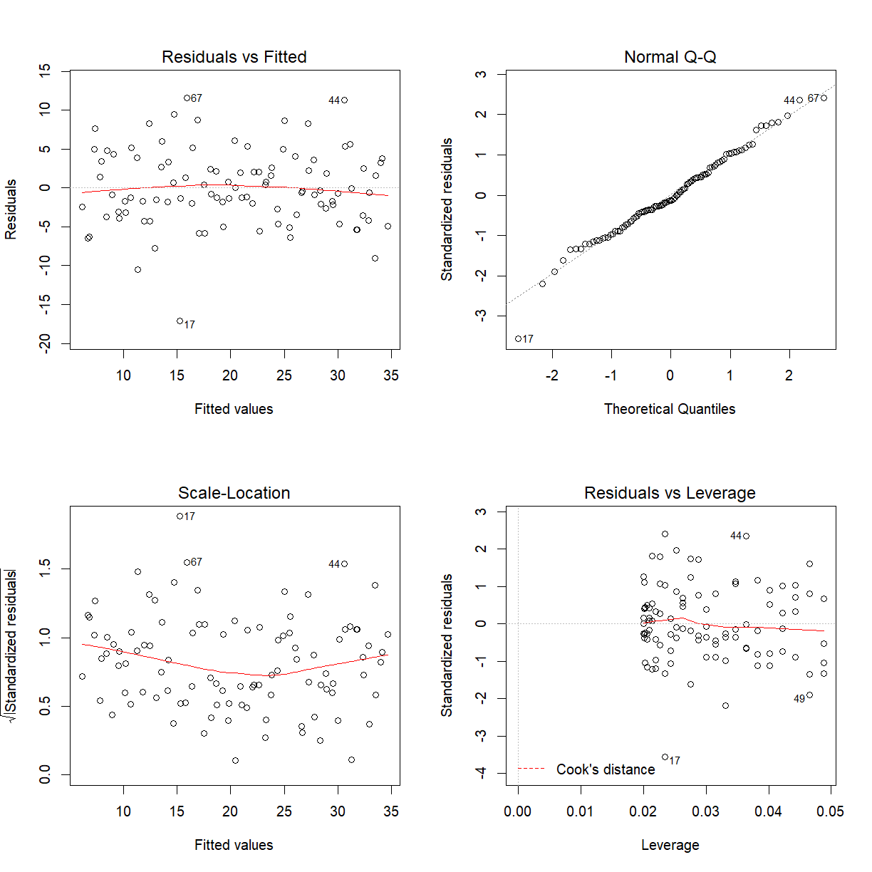
The Residuals vs Leverage ($h_{ii}$) plot can be used to see if you have any points with high
leverage. To actually identify the points use hatvalues(fit) where fit is whatever name you
gave to the model fitted to the data.
Leverage is a measure of how far away the independent variable values of an observation are
from those of the other observations
https://en.wikipedia.org/wiki/Leverage_(statistics)
One rule of thumb for identifying such points is when
We have $n=100$ and $p=2$ so high leverage points will have $h_{ii}>2\frac{(2+1)}{100}=0.06.$ There are no high leverage points under the model fitted.
Influential points are captured by Cook’s distance ($D_i$). An influential observation is an observation if it was removed the regression parameter estimates could be quite different. Such points are said to have high influence.
According to Cook and Weisberg we flag a case as influential if $D_i\geq F_{p+1,n-p-1;0.50}$. For this example all Cook’s distances are close to zero so appears that there are no influential points.
The following can be used to obtain Cook’s Distances.
library(car)

cooks.distance(mass_fit2)
           1            2            3            4            5
1.491363e-02 2.714110e-02 2.203842e-02 8.236742e-03 1.047932e-03
           6            7            8            9           10
1.119823e-02 4.391635e-02 3.386806e-02 1.075475e-01 7.001717e-03
          11           12           13           14           15
9.366549e-02 4.016974e-03 1.165020e-02 1.624058e-01 1.044987e-01
          16           17           18           19           20
1.840585e-05 1.209214e-01 1.045333e-01 6.708925e-02 5.233727e-02
          21           22
2.204762e-02 1.522339e-02
To get $D_i\geq F_{p+1,n-p-1;0.50}$ use qf(.5, df1 = p+1, df2 = n-p-1) in R where you
substitute the number values of df1 and df2.
4. Categorical Predictors
To fit models with categorical predictors with more than two values (levels) we need to use the
lm command in R.
Example: BMD Data set
We have a sample of n=122 post-menopausal women, who took part in a clinical trial of hormone replacement therapy (HRT). The following variables were measured at the start of the trial:
BMD: Bone mineral density at the spine (g/cm²)
BMI: Body Mass Index (kg/m²)
AGE: Years
CALCIUM: Daily calcium intake (mg)
WTKG: Weight (kg)
HTCM: Height (cm)
MENOPYRS: Number of years since menopause
SMKCODE: Smoking status (1=none, 2= 1-10 cigarettes/day, 3= >10 cigarettes/day)
PARITY: Number of children
ALCOHOL: Alcohol intake (1= none, 2= ≤1 drink/day, 3= 2-3 drinks/day, 4= ≥4 drinks/day)
TRTPRV: Previous HRT (0=no, 1=yes)
AGEMENOP: Age at menopause
BMI_CAT: BMI category (1=underweight, 2=normal, 3=overweight, 4=obese, 5=very obese)
OSTEOFAM: Family history of osteoporosis (0=no, 1=yes)
The study was undertaken to assess the effect of HRT on bone mineral density; at the start of the trial, it is of interest to explain the relationship of BMD with the covariates.
The predictor TRTPRV takes on the value 0 if the subject had not previously taken hormone
replacement therapy (HRT), and 1 if she had.
The regression of BMD against BMI and TRTPRV gives:
bmd <- read_csv(file.path("..", "data", "BMD.csv"))
names(bmd) <- c("BMD", "BMI", "AGE", "CALCIUM", "WTKG", "HTCM", "MENOPYRS", "SMKCODE", "PARITY",
    "ALCOHOL", "TRTPRV", "AGEMENOP", "BMI_CAT", "OSTEOFAM")
bmd_fit <- lm(BMD ~ BMI + TRTPRV, data = bmd)

summary(bmd_fit)
Call:
lm(formula = BMD ~ BMI + TRTPRV, data = bmd)

Residuals:
     Min       1Q   Median       3Q      Max
-0.32088 -0.08494  0.00583  0.09239  0.38783

Coefficients:
            Estimate Std. Error t value Pr(>|t|)
(Intercept) 0.945730   0.076010  12.442   <2e-16 ***
BMI         0.005948   0.002867   2.075   0.0402 *
TRTPRV      0.032468   0.028704   1.131   0.2603
---
Signif. codes:  0 '***' 0.001 '**' 0.01 '*' 0.05 '.' 0.1 ' ' 1

Residual standard error: 0.1446 on 119 degrees of freedom
Multiple R-squared:  0.04411,	Adjusted R-squared:  0.02805
F-statistic: 2.746 on 2 and 119 DF,  p-value: 0.06826
TRTPRV is not significant (p=0.260), but let’s consider what the regression is telling us.
If TRTPRV = 0:
If TRTPRV = 1:
In other words, having TRTPRV = 1 results in an increase in the predicted value of BMD of
0.03247 g/cm².
Note that the values of 0 and 1 assigned to TRTPRV are arbitrary, and any other coding would
produce the same fitted values.
TRTPRV is a categorical predictor, or factor, with two levels. What happens when there are
more then two levels? Consider the predictor SMKCODE:
If we regress BMD on SMKCODE we get:
bmd_smoke_fit <- lm(BMD ~ SMKCODE, data = bmd)

summary(bmd_smoke_fit)
Call:
lm(formula = BMD ~ SMKCODE, data = bmd)

Residuals:
     Min       1Q   Median       3Q      Max
-0.32688 -0.09233  0.00366  0.10306  0.41163

Coefficients:
            Estimate Std. Error t value Pr(>|t|)
(Intercept)  1.18137    0.02970  39.782  < 2e-16 ***
SMKCODE     -0.05710    0.02117  -2.697  0.00801 **
---
Signif. codes:  0 '***' 0.001 '**' 0.01 '*' 0.05 '.' 0.1 ' ' 1

Residual standard error: 0.143 on 120 degrees of freedom
Multiple R-squared:  0.05714,	Adjusted R-squared:  0.04929
F-statistic: 7.273 on 1 and 120 DF,  p-value: 0.008007
SMKCODE=1: $BMD_i= 1.18-0.0571\times 1 =1.1229$
SMKCODE=2: $BMD_i=1.18-0.0571\times 2 = 1.0658$
SMKCODE=3: $BMD_i = 1.18-0.0571 \times 3=1.0087$
This means that there is a predicted decrease in BMD of 0.0571 g/cm² when SMKCODE changes
from 1 to 2, and from 2 to 3. This doesn’t make much sense: why should there be an equal
difference in mean BMD between non-smokers and moderate smokers, as between moderate and heavy
smokers?
If we had used different a coding for SMKCODE, we would have obtained a totally different
answer. This makes no sense at all. What we need is a model which recognises that the levels of
a categorical variable are not to be taken literally as numerical values, but rather as
indicators of different states that the variable can be in. For this we need the concept of an
indicator variable.
Indicator variables
Going back to the BMD smoking variable, we define three indicator variables $S_1$, $S_2$ and
$S_3$:
The values of $S_1$, $S_2$ and $S_3$ will then be as follows:
We can then include $S_1$, $S_2$ and $S_3$ in the model. The problem with this approach is
collinearity. We will always have for i-th subject: $S_{i1}+S_{i2}+S_{i3}=1$,
which means there is a perfect collinearity between the indicator variables. Another way to
think of this is that we are giving the model redundant information: for example, for the i-th
subject, if we have $S_{i1}=0$ and $S_{i2}=0$ then we know that we must have $S_{i3}=1$.
We only need to provide two bits of information about SMKCODE in order to convey all of the
information. We leave out one of the indicator variables, and the level of the categorical
variable corresponding to the indicator variable which we leave out, is called the
referent category.
bmd_smoke_fact_fit <- lm(BMD ~ factor(SMKCODE), data = bmd)

summary(bmd_smoke_fact_fit)
Call:
lm(formula = BMD ~ factor(SMKCODE), data = bmd)

Residuals:
     Min       1Q   Median       3Q      Max
-0.33018 -0.08980  0.00036  0.09505  0.40832

Coefficients:
                 Estimate Std. Error t value Pr(>|t|)
(Intercept)       1.12758    0.01412  79.835  < 2e-16 ***
factor(SMKCODE)2 -0.12711    0.04706  -2.701  0.00792 **
factor(SMKCODE)3 -0.08718    0.04507  -1.934  0.05544 .
---
Signif. codes:  0 '***' 0.001 '**' 0.01 '*' 0.05 '.' 0.1 ' ' 1

Residual standard error: 0.1419 on 119 degrees of freedom
Multiple R-squared:  0.07856,	Adjusted R-squared:  0.06307
F-statistic: 5.073 on 2 and 119 DF,  p-value: 0.007689
The referrent category is $S_1$, non-smoker.
Another way of looking at the problem
We have performed an analysis to determine whether Smoking (a categorical variable or factor) is a significant predictor of BMD. An appropriate visual display is the box plot:
boxplot(BMD ~ SMKCODE, data = bmd)
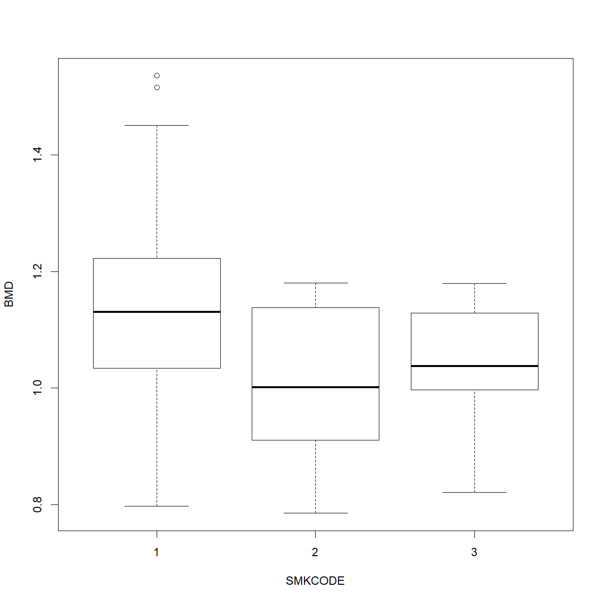
in which we can see the lower BMDs of smokers. This suggests another method of analysis: one-way analysis of variance. The model is
where $Y_{ij} =$ BMD of i-th subject in smoking group j
$\mu =$ Overall mean BMD
$\alpha_j=$ Effect of smoking group j
$n_j=$ Number of subjects in smoking group j
anova(bmd_smoke_fact_fit)
Analysis of Variance Table

Response: BMD
                 Df  Sum Sq  Mean Sq F value   Pr(>F)
factor(SMKCODE)   2 0.20441 0.102204  5.0727 0.007689 **
Residuals       119 2.39759 0.020148
---
Signif. codes:  0 '***' 0.001 '**' 0.01 '*' 0.05 '.' 0.1 ' ' 1
5.1 ANALYSIS OF COVARIANCE
A regression based on a single, categorical predictor is equivalent to a one-way ANOVA. A regression based on more categorical variables as predictors (say m of them) would have been equivalent to an m-way ANOVA. Once we include categorical predictors in the regression framework, by using indicator variables, there is nothing stopping us from also including one or more covariates (or continuous predictors) in the model. Say we have one covariate ($X$) and one categorical predictor ($S$), which has $k$ levels. Assuming that the last ($k$-th) level of $S$ is the referent category, a possible model is
$\varepsilon_i \sim N(0,\sigma^2)$ independently $i=1,\ldots,n$
What (1) is assuming is that the slope of the relationship between $y$ and $x$ is $\beta_1$, irrespective of the value of $S$. This may be depicted, for $k=3$, as:
x <- c(0, 1, 2, 3, 4, 5, 6, 7, 8, 9, 10)
y <- 13.4 + 0.623 * x
example1 <- data.frame(x, y)

ggplot(data = example1, aes(x = x, y = y)) +
    geom_point() +
    geom_abline(intercept = 12.4, slope = 0.623, col = "blue") +
    geom_abline(intercept = 13.4, slope = 0.623) +
    geom_abline(intercept = 14.4, slope = 0.623, col = "red")
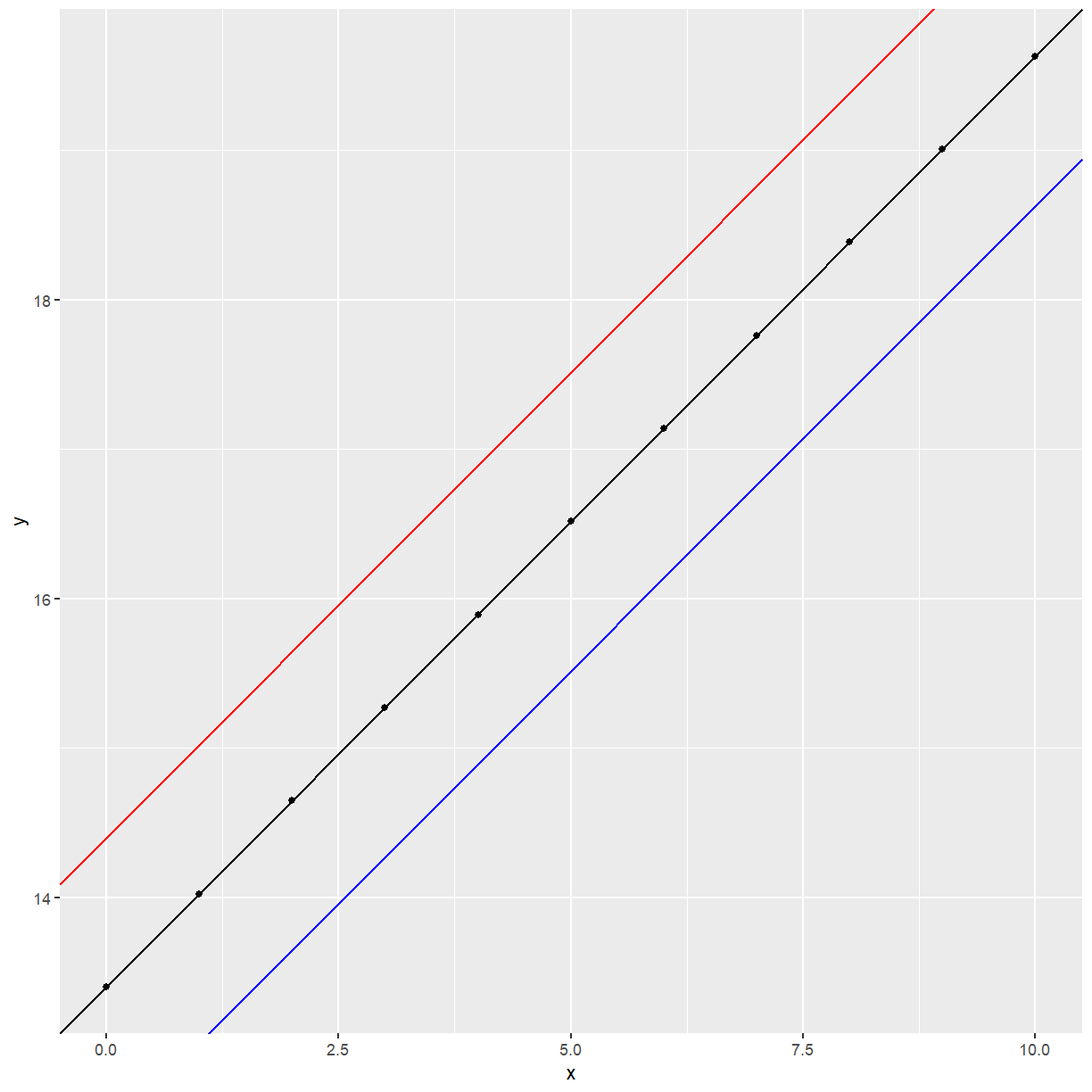
We say here that there is no interaction between X and S.
Another possible scenario is:
x <- c(0, 1, 2, 3, 4, 5, 6, 7, 8, 9, 10)
y <- 13.4 + 1.623 * x
example2 <- data.frame(x, y)

ggplot(data = example2, aes(x = x, y = y)) +
    geom_point() +
    geom_abline(intercept = 12.4, slope = 0.623, col = "blue") +
    geom_abline(intercept = 13.4, slope = 1.623) +
    geom_abline(intercept = 14.4, slope = 0.23, col = "red")
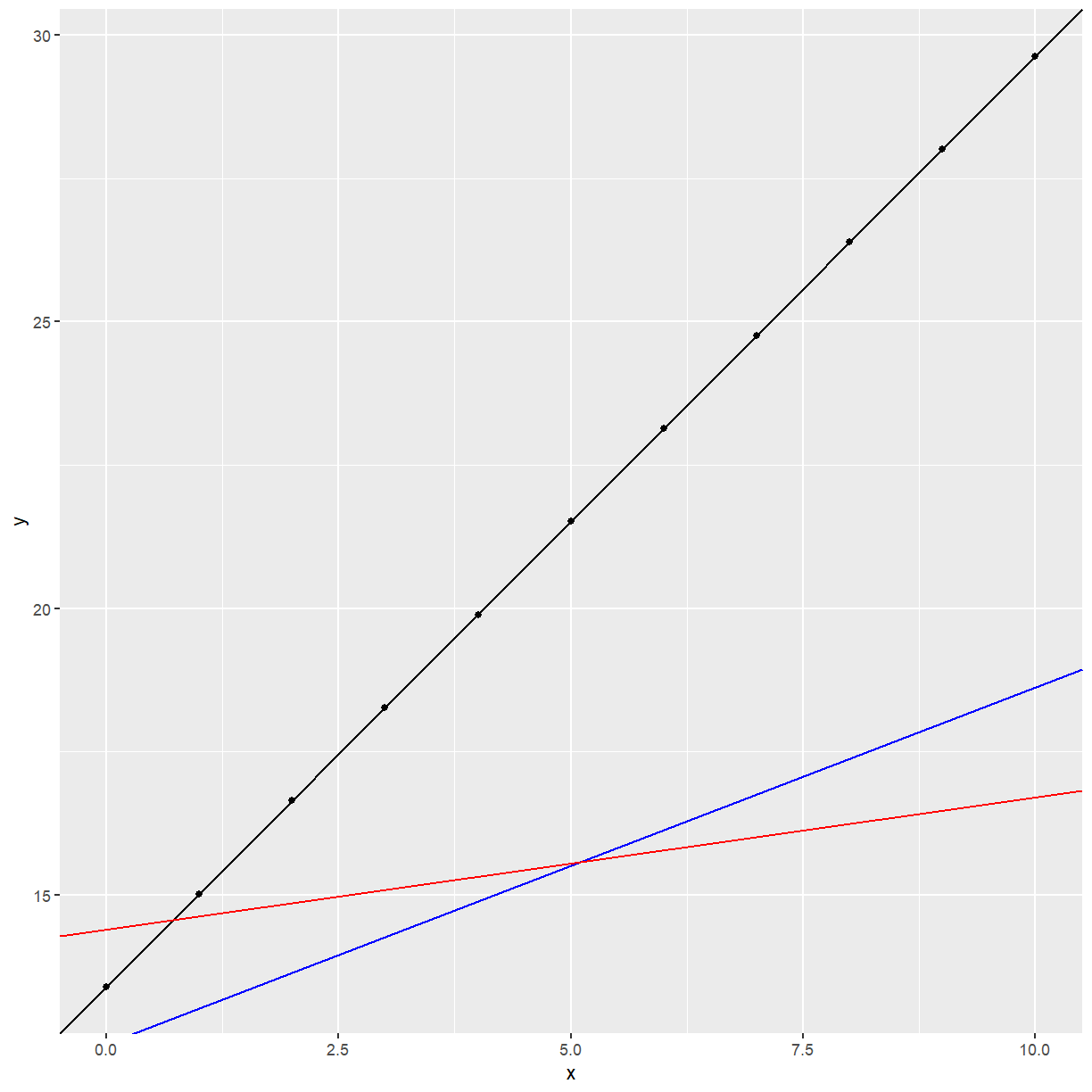
The slope of the relationship between $y$ and $x$ depends on the value of $S$.
This is formulated as follows:
Rewrite as
We have differential slopes for different levels of $S$. For the referent category $k$, the slope is $\beta_1$.
No interaction hypothesis:
No effect of S hypothesis assuming no interaction:
BMD example
Body mass index (BMI) is an important predictor of bone mineral density (BMD). It is a simple matter to include BMI in the model. The following is the model with no interaction, i.e. the same slope between BMD and BMI, irrespective of the subject’s smoking status:
where
$BMI_i$ = body mass index of i-th subject and other definitions are as for model (1). The results are
bmd_bmi_smoke_fit <- lm(BMD ~ BMI + factor(SMKCODE), data = bmd)

summary(bmd_bmi_smoke_fit)
Call:
lm(formula = BMD ~ BMI + factor(SMKCODE), data = bmd)

Residuals:
     Min       1Q   Median       3Q      Max
-0.31668 -0.08025  0.00546  0.09665  0.39288

Coefficients:
                  Estimate Std. Error t value Pr(>|t|)
(Intercept)       0.986226   0.074111  13.307   <2e-16 ***
BMI               0.005428   0.002795   1.942   0.0545 .
factor(SMKCODE)2 -0.126571   0.046518  -2.721   0.0075 **
factor(SMKCODE)3 -0.078738   0.044763  -1.759   0.0812 .
---
Signif. codes:  0 '***' 0.001 '**' 0.01 '*' 0.05 '.' 0.1 ' ' 1

Residual standard error: 0.1403 on 118 degrees of freedom
Multiple R-squared:  0.1071,	Adjusted R-squared:  0.0844
F-statistic: 4.718 on 3 and 118 DF,  p-value: 0.003806
anova(bmd_bmi_smoke_fit)
Analysis of Variance Table

Response: BMD
                 Df  Sum Sq  Mean Sq F value   Pr(>F)
BMI               1 0.08804 0.088044  4.4717 0.036566 *
factor(SMKCODE)   2 0.19062 0.095311  4.8408 0.009538 **
Residuals       118 2.32333 0.019689
---
Signif. codes:  0 '***' 0.001 '**' 0.01 '*' 0.05 '.' 0.1 ' ' 1
The fitted model is
Interpretation of parameters:
The predicted effect on BMD of an increase of 1 kg/m² of BMI, is a increase of 0.005 g/cm².
The predicted effect on BMD of a person being a moderate smoker, compared with a non-smoker, is a decrease of 0.127 g/cm².
The predicted effect on BMD of a person being a heavy smoker, compared with a non-smoker, is a decrease of 0.079 g/cm².
The model with interaction is
bmd_bmi_smoke_fit_int <- lm(BMD ~ BMI * factor(SMKCODE), data = bmd)

summary(bmd_bmi_smoke_fit_int)
Call:
lm(formula = BMD ~ BMI * factor(SMKCODE), data = bmd)

Residuals:
     Min       1Q   Median       3Q      Max
-0.31624 -0.08058  0.00551  0.09204  0.39303

Coefficients:
                      Estimate Std. Error t value Pr(>|t|)
(Intercept)           0.981566   0.079424  12.359   <2e-16 ***
BMI                   0.005607   0.003002   1.868   0.0643 .
factor(SMKCODE)2     -0.251757   0.265309  -0.949   0.3446
factor(SMKCODE)3      0.259077   0.343809   0.754   0.4526
BMI:factor(SMKCODE)2  0.004827   0.010065   0.480   0.6324
BMI:factor(SMKCODE)3 -0.013786   0.013880  -0.993   0.3227
---
Signif. codes:  0 '***' 0.001 '**' 0.01 '*' 0.05 '.' 0.1 ' ' 1

Residual standard error: 0.1407 on 116 degrees of freedom
Multiple R-squared:  0.1169,	Adjusted R-squared:  0.0788
F-statistic:  3.07 on 5 and 116 DF,  p-value: 0.01222
anova(bmd_bmi_smoke_fit_int)
Analysis of Variance Table

Response: BMD
                     Df  Sum Sq  Mean Sq F value   Pr(>F)
BMI                   1 0.08804 0.088044  4.4445 0.037166 *
factor(SMKCODE)       2 0.19062 0.095311  4.8114 0.009831 **
BMI:factor(SMKCODE)   2 0.02542 0.012710  0.6416 0.528309
Residuals           116 2.29791 0.019810
---
Signif. codes:  0 '***' 0.001 '**' 0.01 '*' 0.05 '.' 0.1 ' ' 1
Model fitted:
Alternatively:
SMKCODE=1: $B\hat{M}D_i=0.98157+0.005607\cdot BMI_i$
SMKCODE=2: $B\hat{M}D_i=0.98157+0.005607\cdot BMI_i-0.2518+0.00483\cdot BMI_i$
$=0.72977+0.010437\cdot BMI_i$
SMKCODE=3: $B\hat{M}D_i=0.98157+0.005607\cdot BMI_i+0.2591-0.01379\cdot BMI_i$
$=1.2407-0.008183\cdot BMI_i$
Interpretation of parameters:
Interaction makes interpretation more complicated.
The predicted effect on BMD of an increase of 1 kg/m² of BMI, is:
-
for a non-smoker: an increase of 0.005607 g/cm²;
-
for a moderate smoker: an increase of 0.010437 g/cm²;
-
for a heavy smoker: a decrease of 0.008183 g/cm².
The predicted effect on BMD of a person being a moderate smoker compared with a non-smoker: $-0.25180+0.00483\cdot BMI_i$
The predicted effect on BMD of a person being a heavy smoker compared with a non-smoker: $0.2591-0.01379\cdot BMI_i$
Test for interaction
Always test for interaction before main effects. If interaction is present then we need to retain the main effects in the model. We want to test
We can do this by looking at the ANOVA of the model we fitted with interaction.
anova(bmd_bmi_smoke_fit_int)
Analysis of Variance Table

Response: BMD
                     Df  Sum Sq  Mean Sq F value   Pr(>F)
BMI                   1 0.08804 0.088044  4.4445 0.037166 *
factor(SMKCODE)       2 0.19062 0.095311  4.8114 0.009831 **
BMI:factor(SMKCODE)   2 0.02542 0.012710  0.6416 0.528309
Residuals           116 2.29791 0.019810
---
Signif. codes:  0 '***' 0.001 '**' 0.01 '*' 0.05 '.' 0.1 ' ' 1
The p-value associated with the interaction term is $0.0095$ which is significant. Only can say if this model assumptions hold:
par(mfrow = c(2, 2))
plot(bmd_bmi_smoke_fit_int)
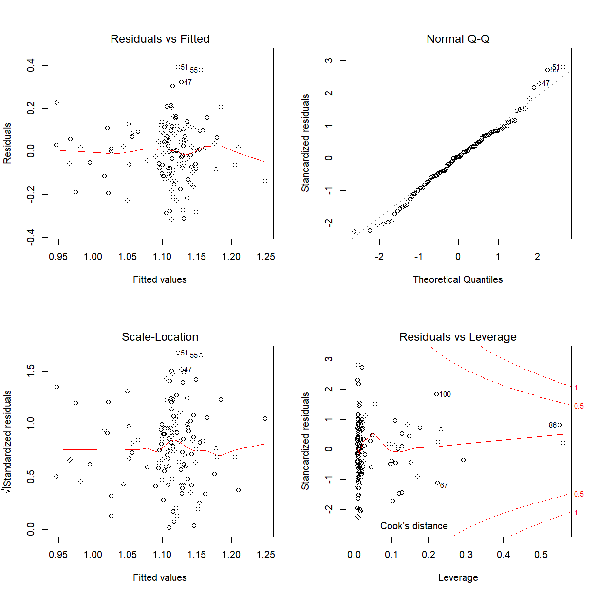
Might be prepared to say the model assumptions hold. Residuals versus Fitted values plot does look like a random scatter about zero and the Normal Q-Q plot looks linear.
We conclude that there is no evidence to confirm a BMI-smoking interaction effect on bone mineral density.
Test for categorical predictor (no interaction present)
In the presence of interaction, we need the main effects to be present in the model and so do not need to check for their significance.
In the absence of interaction, we test for the overall significance of the categorical predictor, again via a multiple partial F-test. (R gives you this when you obtain the ANOVA of the model fitted without an interaction term whit was fit above.)
The full model is
We test:
We can do this by looking at the ANOVA of the model we fitted with no interaction earlier.
anova(bmd_bmi_smoke_fit)
Analysis of Variance Table

Response: BMD
                 Df  Sum Sq  Mean Sq F value   Pr(>F)
BMI               1 0.08804 0.088044  4.4717 0.036566 *
factor(SMKCODE)   2 0.19062 0.095311  4.8408 0.009538 **
Residuals       118 2.32333 0.019689
---
Signif. codes:  0 '***' 0.001 '**' 0.01 '*' 0.05 '.' 0.1 ' ' 1
The p-value associated with the model is $0.0095$ which is significant. We strongly reject $H_0$ in favour of $H_1$. We conclude that Smoking is a significant predictor of BMD, after correcting (or controlling) for Body Mass Index. We only can say if this model assumptions hold:
par(mfrow = c(2, 2))
plot(bmd_bmi_smoke_fit)
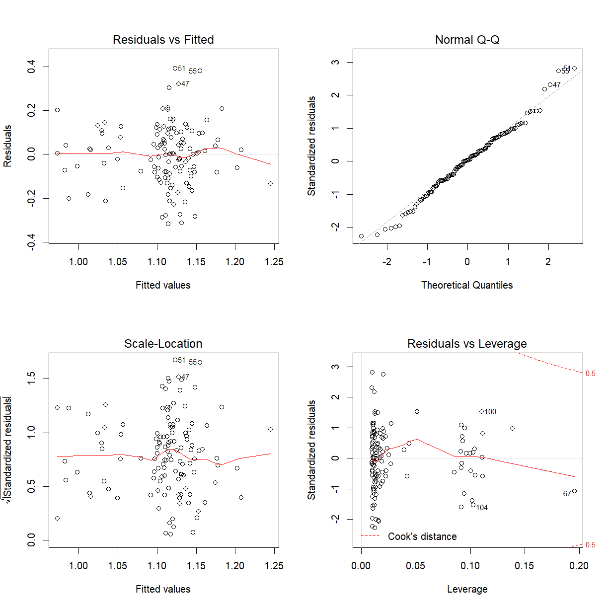
Tests for individual coefficients
summary(bmd_bmi_smoke_fit)
Call:
lm(formula = BMD ~ BMI + factor(SMKCODE), data = bmd)

Residuals:
     Min       1Q   Median       3Q      Max
-0.31668 -0.08025  0.00546  0.09665  0.39288

Coefficients:
                  Estimate Std. Error t value Pr(>|t|)
(Intercept)       0.986226   0.074111  13.307   <2e-16 ***
BMI               0.005428   0.002795   1.942   0.0545 .
factor(SMKCODE)2 -0.126571   0.046518  -2.721   0.0075 **
factor(SMKCODE)3 -0.078738   0.044763  -1.759   0.0812 .
---
Signif. codes:  0 '***' 0.001 '**' 0.01 '*' 0.05 '.' 0.1 ' ' 1

Residual standard error: 0.1403 on 118 degrees of freedom
Multiple R-squared:  0.1071,	Adjusted R-squared:  0.0844
F-statistic: 4.718 on 3 and 118 DF,  p-value: 0.003806
Test for the significance of $\gamma_j$, compared with the referent category.
For $H_0:\gamma_2=0$ we have $\gamma_2$ significant (p=0.0075) and for $H_0:\gamma_3=0$, we have $\gamma_3$ not significant (p=0.081).
We conclude that moderate smokers have mean BMD levels significantly lower than non-smokers, but that heavy smokers’ mean BMD levels are not significantly different from non-smokers. [The numbers of heavy smokers in the sample was small, making the detection of a significant difference unlikely, even if there was a significant difference in the population.]
Caution: Here we have performed two hypothesis tests, both at a 5% level of significance. Is the overall significance of our conclusion still 5%? If not, is it greater than or less than 5%?
Referent category revisited
A sensible choice for referent category will be a category which:
- for numerical stability: is not sparse; has a reasonable number of observations; and
- is a sensible point of reference in the context of the problem.
In the BMD example, we have the following frequencies for Smkcode:
There are few moderate and heavy smokers relative to non-smokers, and a comparison with reference to non-smokers makes sense.
Transformation of variables will be covered in the last Exercise for this lesson.
Key Points